Estimation of tree height using GEDI dataset - Random Forest prediction
Jupyterlab setup and libraries retrieving [Just for UBUNTU 24.04]
To run this lesson properly on osboxes.org you need to have a clean install of jupyterlab using the command line. If you didn’t do it for the previous lesson (Python data analysis or Python geospatial analysis), do it for this one, directly on the terminal:
pipx uninstall jupyterlab
pipx install --system-site-packages jupyterlab
and just after that, you can procede to install python libraries, using the apt install always in the terminal:
sudo apt install python3-numpy python3-pandas python3-sklearn python3-matplotlib python3-rasterio python3-geopandas python3-seaborn python3-skimage python3-xarray
Jupyterlab setup and libraries retrieving [Just for OSGEOLIVE16]
In order to run this notebook you need to run this command lines in your terminal:
source $HOME/venv/bin/activate
sudo apt update
sudo apt install python3-pip
pip3 install pyspatialml
after that all other needed libraries directly on jupyter with the magic lines (!):
!pip3 install "pandas>=2.2.2,<3.0.0" "numpy>=1.26.4,<2.0.0" "rasterio>=1.3.10,<2.0.0" "scikit-learn>=1.4.2,<2.0.0" "scipy>=1.13.0,<2.0.0" "matplotlib>=3.9.0,<4.0.0" "xarray>=2024.1.0,<2025.0.0"
Data retrieving (>3GB)
cd  /media/sf_LVM_shared/my_SE_data/exercise/
pipx install gdown
~/.local/bin/gdown 1Y60EuLsfmTICTX-U_FxcE1odNAf04bd-
tar -xvzf tree_height.tar.gz
Open the notebook lesson
Open the lesson using the CL
cd /media/sf_LVM_shared/my_SE_data/exercise
jupyter-lab Tree_Height_03RF_pred_SM.ipynb
Model definition
y ~ f ( a*x1 + b*x2 + c*x3 + …) + ε,
where y is the response variable, the x’s are predictor variables, and ε is the associated error.
Different types of models
Parametric models – make assumptions about the underlying distribution of the data:
Maximum likelihood classification,
Discriminant analysis,
General linear models (ex. linear regression)
Nonparametric models – make no assumptions about the underlying data distributions:
Generalized additive models,
Support Vector Machine,
Artificial neural networks,
Random Forest
Random forest
Random forest is a Supervised Machine Learning Algorithm that is used widely in Classification (containing categorical variables) and Regression (response continuous variables) problems. It builds decision trees on different samples and takes their majority vote for classification and average in case of regression.
One of the most important features of the Random Forest Algorithm is that it can handle continuous and categorical variables predictors without any assamption on their data distribution, dimension, and even if the predictors are autocorrelated.
Steps involved in random forest algorithm:
Step 1: In Random forest n number of random records are taken from the data set having k number of records.
Step 2: Individual decision trees are constructed for each sample.
- Step 3: Each decision tree will generate an output.
Step 4: Final output is considered based on Majority Voting or Averaging for Classification and regression respectively.
(source https://www.analyticsvidhya.com/blog/2021/06/understanding-random-forest/)

Random Forest test
In this exercise we will use Random Forest Regression algorithm with the sklearn python package to estimage the tree height. In last step, we will see how it was possible to have a prediction on a raster using Pyspatialml library (now deprecated) and how we can to the same but using the updated more robust Xarray and Rasterio libraries for the spatial prediction on the raster files.
[2]:
import pandas as pd
import numpy as np
import rasterio
from rasterio import *
from rasterio.plot import show
from sklearn.ensemble import RandomForestRegressor
from sklearn.model_selection import train_test_split,GridSearchCV
from sklearn.pipeline import Pipeline
from scipy.stats import pearsonr
import matplotlib.pyplot as plt
plt.rcParams["figure.figsize"] = (10,6.5)
Data analysis
Before everything we need to import the raw data, within the extracted predictors and show whole the data distribution
[3]:
predictors = pd.read_csv("tree_height/txt/eu_x_y_height_predictors_select.txt", sep=" ",  index_col=False)
pd.set_option('display.max_columns',None)

# change column name
predictors = predictors.rename({'dev-magnitude':'devmagnitude'} , axis='columns')
predictors.head(10)
[3]:
| ID | X | Y | h | BLDFIE_WeigAver | CECSOL_WeigAver | CHELSA_bio18 | CHELSA_bio4 | convergence | cti | devmagnitude | eastness | elev | forestheight | glad_ard_SVVI_max | glad_ard_SVVI_med | glad_ard_SVVI_min | northness | ORCDRC_WeigAver | outlet_dist_dw_basin | SBIO3_Isothermality_5_15cm | SBIO4_Temperature_Seasonality_5_15cm | treecover | |
|---|---|---|---|---|---|---|---|---|---|---|---|---|---|---|---|---|---|---|---|---|---|---|---|
| 0 | 1 | 6.050001 | 49.727499 | 3139.00 | 1540 | 13 | 2113 | 5893 | -10.486560 | -238043120 | 1.158417 | 0.069094 | 353.983124 | 23 | 276.871094 | 46.444092 | 347.665405 | 0.042500 | 9 | 780403 | 19.798992 | 440.672211 | 85 |
| 1 | 2 | 6.050002 | 49.922155 | 1454.75 | 1491 | 12 | 1993 | 5912 | 33.274361 | -208915344 | -1.755341 | 0.269112 | 267.511688 | 19 | -49.526367 | 19.552734 | -130.541748 | 0.182780 | 16 | 772777 | 20.889412 | 457.756195 | 85 |
| 2 | 3 | 6.050002 | 48.602377 | 853.50 | 1521 | 17 | 2124 | 5983 | 0.045293 | -137479792 | 1.908780 | -0.016055 | 389.751160 | 21 | 93.257324 | 50.743652 | 384.522461 | 0.036253 | 14 | 898820 | 20.695877 | 481.879700 | 62 |
| 3 | 4 | 6.050009 | 48.151979 | 3141.00 | 1526 | 16 | 2569 | 6130 | -33.654274 | -267223072 | 0.965787 | 0.067767 | 380.207703 | 27 | 542.401367 | 202.264160 | 386.156738 | 0.005139 | 15 | 831824 | 19.375000 | 479.410278 | 85 |
| 4 | 5 | 6.050010 | 49.588410 | 2065.25 | 1547 | 14 | 2108 | 5923 | 27.493824 | -107809368 | -0.162624 | 0.014065 | 308.042786 | 25 | 136.048340 | 146.835205 | 198.127441 | 0.028847 | 17 | 796962 | 18.777500 | 457.880066 | 85 |
| 5 | 6 | 6.050014 | 48.608456 | 1246.50 | 1515 | 19 | 2124 | 6010 | -1.602039 | 17384282 | 1.447979 | -0.018912 | 364.527100 | 18 | 221.339844 | 247.387207 | 480.387939 | 0.042747 | 14 | 897945 | 19.398880 | 474.331329 | 62 |
| 6 | 7 | 6.050016 | 48.571401 | 2938.75 | 1520 | 19 | 2169 | 6147 | 27.856503 | -66516432 | -1.073956 | 0.002280 | 254.679596 | 19 | 125.250488 | 87.865234 | 160.696777 | 0.037254 | 11 | 908426 | 20.170450 | 476.414520 | 96 |
| 7 | 8 | 6.050019 | 49.921613 | 3294.75 | 1490 | 12 | 1995 | 5912 | 22.102139 | -297770784 | -1.402633 | 0.309765 | 294.927765 | 26 | -86.729492 | -145.584229 | -190.062988 | 0.222435 | 15 | 772784 | 20.855963 | 457.195404 | 86 |
| 8 | 9 | 6.050020 | 48.822645 | 1623.50 | 1554 | 18 | 1973 | 6138 | 18.496584 | -25336536 | -0.800016 | 0.010370 | 240.493759 | 22 | -51.470703 | -245.886719 | 172.074707 | 0.004428 | 8 | 839132 | 21.812290 | 496.231110 | 64 |
| 9 | 10 | 6.050024 | 49.847522 | 1400.00 | 1521 | 15 | 2187 | 5886 | -5.660453 | -278652608 | 1.477951 | -0.068720 | 376.671143 | 12 | 277.297363 | 273.141846 | -138.895996 | 0.098817 | 13 | 768873 | 21.137711 | 466.976685 | 70 |
[6]:
print("NUMBER OF ROWS:",len(predictors))
NUMBER OF ROWS: 1267239
To deeper analyze data distribution its always good to plot them
[7]:
bins = np.linspace(min(predictors['h']),max(predictors['h']),100)
plt.hist((predictors['h']),bins,alpha=0.8);

In this way we can see where the date spans to, and detect outliers.
Indeed, in this case we’re gonna select only trees with height below 70m (because in this area, the highest tree detected in germany was 67m https://visit.freiburg.de/en/attractions/waldtraut-germany-s-tallest-tree).
And we procede sampling just 100K points out of the 1.2M, to train a lighter model.
[24]:
predictors_sel = predictors.loc[(predictors['h'] < 7000)  ].sample(100000)

# add a height column in meter
predictors_sel.insert ( 4, 'hm' ,  predictors_sel['h']/100 )

# overlook
predictors_sel.head(10)
[24]:
| ID | X | Y | h | hm | BLDFIE_WeigAver | CECSOL_WeigAver | CHELSA_bio18 | CHELSA_bio4 | convergence | cti | devmagnitude | eastness | elev | forestheight | glad_ard_SVVI_max | glad_ard_SVVI_med | glad_ard_SVVI_min | northness | ORCDRC_WeigAver | outlet_dist_dw_basin | SBIO3_Isothermality_5_15cm | SBIO4_Temperature_Seasonality_5_15cm | treecover | |
|---|---|---|---|---|---|---|---|---|---|---|---|---|---|---|---|---|---|---|---|---|---|---|---|---|
| 81999 | 82000 | 6.349125 | 49.644223 | 2659.75 | 26.5975 | 1530 | 16 | 2272 | 5931 | 21.476559 | -141539392 | 1.694310 | -0.040122 | 331.223236 | 23 | 631.313477 | 214.736084 | 365.218750 | 0.057163 | 25 | 717991 | 18.626610 | 451.421082 | 86 |
| 965362 | 965363 | 9.012956 | 49.690358 | 2689.50 | 26.8950 | 1536 | 12 | 2137 | 6537 | 15.065849 | 120771872 | -1.399779 | -0.072601 | 242.992401 | 26 | 353.459473 | 270.740967 | 220.016357 | 0.026610 | 9 | 719463 | 20.024574 | 492.804718 | 75 |
| 1236259 | 1236260 | 9.801078 | 49.395159 | 2572.00 | 25.7200 | 1528 | 16 | 2238 | 6472 | 16.836056 | -162671216 | 0.910004 | -0.033257 | 418.785919 | 20 | -54.990723 | 61.513428 | 257.196045 | 0.045267 | 8 | 806762 | 19.990988 | 525.202148 | 82 |
| 1115641 | 1115642 | 9.382723 | 49.106039 | 2370.00 | 23.7000 | 1513 | 15 | 2407 | 6637 | -24.503428 | -231658992 | -0.858004 | -0.064393 | 267.034180 | 4 | 536.372314 | 470.607422 | 432.341064 | 0.030045 | 6 | 784144 | 19.837236 | 517.255615 | 29 |
| 215407 | 215408 | 6.773116 | 49.944617 | 1392.00 | 13.9200 | 1515 | 12 | 1952 | 6118 | 26.732821 | -193019280 | 0.534557 | -0.005609 | 300.268585 | 22 | -162.502686 | -200.892090 | -412.381104 | 0.056135 | 15 | 666767 | 19.065788 | 437.629272 | 74 |
| 939859 | 939860 | 8.948157 | 49.643079 | 2365.25 | 23.6525 | 1481 | 13 | 2466 | 6341 | -10.630081 | -171884224 | 1.417312 | -0.121560 | 400.390808 | 26 | -52.929199 | -124.971191 | -149.944336 | 0.015808 | 9 | 737709 | 19.441750 | 473.700439 | 89 |
| 157727 | 157728 | 6.620174 | 49.837913 | 3160.75 | 31.6075 | 1536 | 13 | 2164 | 6052 | -57.077930 | -253935056 | 1.182596 | -0.038630 | 343.578552 | 24 | 178.370117 | 86.893066 | 392.301758 | -0.081356 | 23 | 675920 | 19.584587 | 443.499878 | 100 |
| 376387 | 376388 | 7.163473 | 49.791920 | 3010.00 | 30.1000 | 1352 | 12 | 2377 | 5621 | -3.525097 | -193161968 | 3.196814 | 0.090454 | 699.986816 | 22 | 435.113525 | 436.794434 | 406.962158 | -0.108846 | 32 | 638925 | 22.397139 | 416.059174 | 87 |
| 426482 | 426483 | 7.277403 | 49.534507 | 277.75 | 2.7775 | 1494 | 15 | 2251 | 6162 | 7.484096 | -268103968 | 0.745217 | 0.029769 | 391.105804 | 14 | -40.088135 | -26.999023 | -72.698975 | 0.078123 | 12 | 641196 | 20.374083 | 485.715973 | 75 |
| 286481 | 286482 | 6.954634 | 48.417400 | 2362.50 | 23.6250 | 1331 | 20 | 3297 | 6108 | 15.627705 | -346475904 | 0.985921 | 0.047404 | 547.931702 | 33 | -2.996826 | -0.247314 | -181.765503 | 0.207945 | 50 | 960411 | 21.377501 | 454.721680 | 95 |
[25]:
print("NUMBER OF ROWS:",len(predictors_sel))
NUMBER OF ROWS: 100000
Now we can see again the data distribution with the same plotting used before
[26]:
bins = np.linspace(min(predictors_sel['hm']),max(predictors_sel['hm']),100)
plt.hist((predictors_sel['hm']),bins,alpha=0.8);

To have a comparison we’ll analyze the The Global Forest Canopy Height, 2019 map. This has been released in 2020 (within a scientific publication https://doi.org/10.1016/j.rse.2020.112165).
The authors used a regression tree model that was calibrated and applied to each individual Landsat GLAD ARD tile (1° × 1°) in a “moving window” mode.
This tree height estimation its available as forestheight.tiff and their extracted values available in the table as forestheight column.
To see how this model performed we can see a correlation plot and its calculated pearson coefficient.
[27]:
plt.rcParams["figure.figsize"] = (8,6)
plt.scatter(predictors['h']/100,predictors['forestheight'])
plt.xlabel('sensed tree height\n (m)')
plt.ylabel('estimated tree height\n (m)')
ident = [0, 50]
plt.plot(ident,ident,'r--')
[27]:
[<matplotlib.lines.Line2D at 0x712ff962c980>]

[28]:
# calculating the pearson correlation index
pearsonr_Publication_Estimation = pearsonr(predictors['h'],predictors['forestheight'])[0]

print("PEARSON CORRELATION COEFFINCENT:", pearsonr_Publication_Estimation)
PEARSON CORRELATION COEFFINCENT: 0.4527925130004339
In this procedure we will try to outperform this model Pearson Correlation Coefficent.
To do that we’re gonna use a more advanced Machine Learning architecture with some more and different enviromental predictors that could better express the ecological asset and the physical conditions.
Data set splitting
To procede we need to split the dataset (predictors_sel) in order to create the response variable table that will be used against the predictors variables (excluding the forestheight predictors).
[29]:
X = predictors_sel.iloc[:,[5,6,7,8,9,10,11,12,13,15,16,17,18,19,20,21,22,23]].values
Y = predictors_sel.iloc[:,4:5].values
feat = predictors_sel.iloc[:,[5,6,7,8,9,10,11,12,13,15,16,17,18,19,20,21,22,23]].columns.values
Its always good to double check that we select the right columns in the right order
[30]:
feat
[30]:
array(['BLDFIE_WeigAver', 'CECSOL_WeigAver', 'CHELSA_bio18',
       'CHELSA_bio4', 'convergence', 'cti', 'devmagnitude', 'eastness',
       'elev', 'glad_ard_SVVI_max', 'glad_ard_SVVI_med',
       'glad_ard_SVVI_min', 'northness', 'ORCDRC_WeigAver',
       'outlet_dist_dw_basin', 'SBIO3_Isothermality_5_15cm',
       'SBIO4_Temperature_Seasonality_5_15cm', 'treecover'], dtype=object)
[31]:
print("RESPONSE VARIABLE DIMENSION:", Y.shape)
RESPONSE VARIABLE DIMENSION: (100000, 1)
[32]:
print("PREDICTING FEATURES DIMENSION:", X.shape)
PREDICTING FEATURES DIMENSION: (100000, 18)
Now we can create 4 different dataset:
2 for model algorithm training (X_train and Y_train)
2 for model testing (X_test and Y_test)
[40]:
X_train, X_test, Y_train, Y_test = train_test_split(X, Y, test_size=0.5, random_state=42)
y_train = np.ravel(Y_train)
y_test = np.ravel(Y_test)
Random Forest default parameters
Random Forest can be implemented using the RandomForestRegressor in scikit-learn
We can procede on training the Random Forest model using its default parameters.
[41]:
rf = RandomForestRegressor(random_state = 42)
rf.get_params()
[41]:
{'bootstrap': True,
 'ccp_alpha': 0.0,
 'criterion': 'squared_error',
 'max_depth': None,
 'max_features': 1.0,
 'max_leaf_nodes': None,
 'max_samples': None,
 'min_impurity_decrease': 0.0,
 'min_samples_leaf': 1,
 'min_samples_split': 2,
 'min_weight_fraction_leaf': 0.0,
 'monotonic_cst': None,
 'n_estimators': 100,
 'n_jobs': None,
 'oob_score': False,
 'random_state': 42,
 'verbose': 0,
 'warm_start': False}
[42]:
rfReg = RandomForestRegressor(min_samples_leaf=50, oob_score=True)
rfReg.fit(X_train, y_train);
dic_pred = {}
dic_pred['train'] = rfReg.predict(X_train)
dic_pred['test'] = rfReg.predict(X_test)
pearsonr_all = [pearsonr(dic_pred['train'],y_train)[0],pearsonr(dic_pred['test'],y_test)[0]]
print("PEARSON CORRELATION COEFFINCENT:", pearsonr_all)
PEARSON CORRELATION COEFFINCENT: [0.6035710046325166, 0.506707480767017]
[45]:
# checking the oob score
print("OUT OF BAG SCORE:", rfReg.oob_score_)
OUT OF BAG SCORE: 0.2625683482738882
Additional resources that can be used to reduce more the oob error can be found at:
https://scikit-learn.org/stable/auto_examples/ensemble/plot_ensemble_oob.html
[52]:
plt.rcParams["figure.figsize"] = (8,6)
plt.scatter(y_train,dic_pred['train'])
plt.xlabel('Training GEDI Height (all dataset)\n (m)')
plt.ylabel('Training Tree Height prediction\n (m)')
ident = [0, 50]
plt.plot(ident,ident,'r--')
[52]:
[<matplotlib.lines.Line2D at 0x712ff7839910>]
[47]:
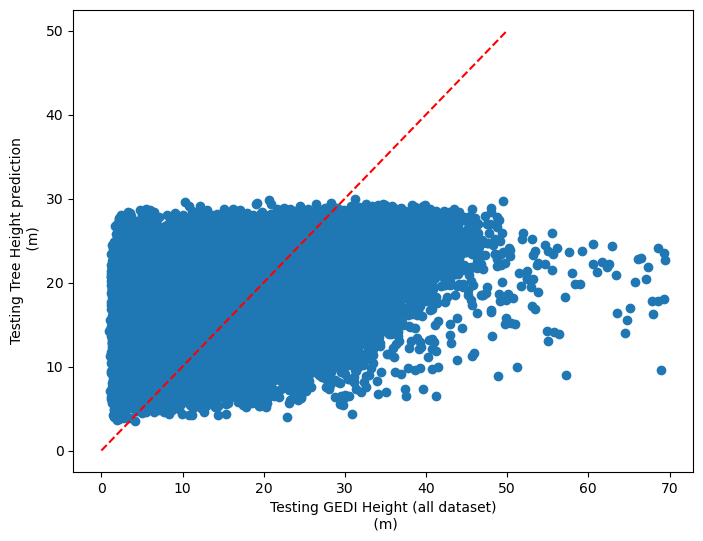
plt.rcParams["figure.figsize"] = (8,6)
plt.scatter(y_test,dic_pred['test'])
plt.xlabel('Testing GEDI Height (all dataset)\n (m)')
plt.ylabel('Testing Tree Height prediction\n (m)')
ident = [0, 50]
plt.plot(ident,ident,'r--')
[47]:
[<matplotlib.lines.Line2D at 0x712ff7a23f50>]

[54]:
impt = [rfReg.feature_importances_, np.std([tree.feature_importances_ for tree in rfReg.estimators_],axis=1)]
ind = np.argsort(impt[0])
[55]:
ind
[55]:
array([ 1, 13,  0,  4,  6,  8, 16,  2, 15,  5, 12,  3, 11,  9, 14,  7, 10,
       17])
To deeper analyze model behaviour in response variable regression we can extract the Feature Importance Ranking
[56]:
plt.rcParams["figure.figsize"] = (6,10)
plt.barh(range(len(feat)),impt[0][ind],color="b", xerr=impt[1][ind], align="center")
plt.yticks(range(len(feat)),feat[ind]);

Model tuning whith Hyperparameters Tweeking
To improve model performance we can use tools like GridSearchCV to find with a recursive search the best combination of all model hyperparameters imployed.
Hyperparameters that were setted as default in the first model run, like:
“max_features”: number of features to consider when looking for the best split.
“max_samples”: number of samples to draw from X to train each base estimator.
“n_estimators”: identify the number of trees that must grow. It must be large enough so that the error is stabilized. Defoult 100.
“max_depth”: max number of levels in each decision tree.
By using this code we can tune up those parameters to improve the algoirithm performance (this code is not runned directly because of its big computational demand as for time and memory perspective)
pipeline = Pipeline([('rf',RandomForestRegressor())])

parameters = {
        'rf__max_features':(3,4,5),
        'rf__max_samples':(0.5,0.6,0.7),
        'rf__n_estimators':(500,1000),
        'rf__max_depth':(50,100,200,300)}

grid_search = GridSearchCV(pipeline,parameters,n_jobs=6,cv=5,scoring='r2',verbose=1)
grid_search.fit(X_train,y_train)


rfReg = RandomForestRegressor(n_estimators=5000,max_features=0.33,max_depth=500,max_samples=0.7,n_jobs=-1,random_state=24 , oob_score = True)
rfReg.fit(X_train, y_train);
dic_pred = {}
dic_pred['train'] = rfReg.predict(X_train)
dic_pred['test'] = rfReg.predict(X_test)
pearsonr_all_tune = [pearsonr(dic_pred['train'],y_train)[0],pearsonr(dic_pred['test'],y_test)[0]]
pearsonr_all_tune

grid_search.best_score_

print ('Best Training score: %0.3f' % grid_search.best_score_)
print ('Optimal parameters:') best_par = grid_search.best_estimator_.get_params()
for par_name in sorted(parameters.keys()):
    print ('\t%s: %r' % (par_name, best_par[par_name]))
Tracking the error rate trend as in https://scikit-learn.org/stable/auto_examples/ensemble/plot_ensemble_oob.html
Features importance ranking shows that the most important variable is treecover followed by Spectral Variability Vegetation Index, and outlet_dist_dw_basin which is a proxy of water accumulation.
Besides eastness and northness describes microclimat condition.
Model tuning with data selection
We can enhance the model performance also by having a wise data selection.
In this case we can have it based on data quality flag (available in the dataset) to select more reilable tree height points.
File storing tree hight (cm) obtained by 6 algorithms, with their associate quality flags. The quality flags can be used to refine and select the best tree height estimation and use it as tree height observation.
a?_95: tree hight (cm) at 95 quintile, for each algorithm
min_rh_95: minimum value of tree hight (cm) ammong the 6 algorithms
max_rh_95: maximum value of tree hight (cm) ammong the 6 algorithms
BEAM: 1-4 coverage beam = lower power (worse) ; 5-8 power beam = higher power (better)
digital_elev: digital mdoel elevation
elev_low: elevation of center of lowest mode
qc_a?: quality_flag for six algorithms quality_flag = 1 (better); = 0 (worse)
se_a?: sensitivity for six algorithms sensitivity < 0.95 (worse); sensitivity > 0.95 (beter )
deg_fg: (degrade_flag) not-degraded 0 (better) ; degraded > 0 (worse)
solar_ele: solar elevation. > 0 day (worse); < 0 night (better)
[57]:
height_6algorithms = pd.read_csv("tree_height/txt/eu_y_x_select_6algorithms_fullTable.txt", sep=" ",  index_col=False)
pd.set_option('display.max_columns',None)
height_6algorithms.head(6)
[57]:
| ID | X | Y | a1_95 | a2_95 | a3_95 | a4_95 | a5_95 | a6_95 | min_rh_95 | max_rh_95 | BEAM | digital_elev | elev_low | qc_a1 | qc_a2 | qc_a3 | qc_a4 | qc_a5 | qc_a6 | se_a1 | se_a2 | se_a3 | se_a4 | se_a5 | se_a6 | deg_fg | solar_ele | |
|---|---|---|---|---|---|---|---|---|---|---|---|---|---|---|---|---|---|---|---|---|---|---|---|---|---|---|---|---|
| 0 | 1 | 6.050001 | 49.727499 | 3139 | 3139 | 3139 | 3120 | 3139 | 3139 | 3120 | 3139 | 5 | 410.0 | 383.72153 | 1 | 1 | 1 | 1 | 1 | 1 | 0.962 | 0.984 | 0.968 | 0.962 | 0.989 | 0.979 | 0 | 17.7 |
| 1 | 2 | 6.050002 | 49.922155 | 1022 | 2303 | 970 | 872 | 5596 | 1524 | 872 | 5596 | 5 | 290.0 | 2374.14110 | 0 | 0 | 0 | 0 | 0 | 0 | 0.948 | 0.990 | 0.960 | 0.948 | 0.994 | 0.980 | 0 | 43.7 |
| 2 | 3 | 6.050002 | 48.602377 | 380 | 1336 | 332 | 362 | 1336 | 1340 | 332 | 1340 | 4 | 440.0 | 435.97781 | 1 | 1 | 1 | 1 | 1 | 1 | 0.947 | 0.975 | 0.956 | 0.947 | 0.981 | 0.968 | 0 | 0.2 |
| 3 | 4 | 6.050009 | 48.151979 | 3153 | 3142 | 3142 | 3127 | 3138 | 3142 | 3127 | 3153 | 2 | 450.0 | 422.00537 | 1 | 1 | 1 | 1 | 1 | 1 | 0.930 | 0.970 | 0.943 | 0.930 | 0.978 | 0.962 | 0 | -14.2 |
| 4 | 5 | 6.050010 | 49.588410 | 666 | 4221 | 651 | 33 | 5611 | 2723 | 33 | 5611 | 8 | 370.0 | 2413.74830 | 0 | 0 | 0 | 0 | 0 | 0 | 0.941 | 0.983 | 0.946 | 0.941 | 0.992 | 0.969 | 0 | 22.1 |
| 5 | 6 | 6.050014 | 48.608456 | 787 | 1179 | 1187 | 761 | 1833 | 1833 | 761 | 1833 | 3 | 420.0 | 415.51581 | 1 | 1 | 1 | 1 | 1 | 1 | 0.952 | 0.979 | 0.961 | 0.952 | 0.986 | 0.975 | 0 | 0.2 |
[58]:
height_6algorithms_sel = height_6algorithms.loc[(height_6algorithms['BEAM'] > 4)
                                            &   (height_6algorithms['qc_a1'] == 1)
                                            &   (height_6algorithms['qc_a2'] == 1)
                                            &   (height_6algorithms['qc_a3'] == 1)
                                            &   (height_6algorithms['qc_a4'] == 1)
                                            &   (height_6algorithms['qc_a5'] == 1)
                                            &   (height_6algorithms['qc_a6'] == 1)
                                            &   (height_6algorithms['se_a1'] > 0.95)
                                            &   (height_6algorithms['se_a2'] > 0.95)
                                            &   (height_6algorithms['se_a3'] > 0.95)
                                            &   (height_6algorithms['se_a4'] > 0.95)
                                            &   (height_6algorithms['se_a5'] > 0.95)
                                            &   (height_6algorithms['se_a6'] > 0.95)
                                            &   (height_6algorithms['deg_fg'] == 0)
                                            &   (height_6algorithms['solar_ele'] < 0)]
[59]:
height_6algorithms_sel
[59]:
| ID | X | Y | a1_95 | a2_95 | a3_95 | a4_95 | a5_95 | a6_95 | min_rh_95 | max_rh_95 | BEAM | digital_elev | elev_low | qc_a1 | qc_a2 | qc_a3 | qc_a4 | qc_a5 | qc_a6 | se_a1 | se_a2 | se_a3 | se_a4 | se_a5 | se_a6 | deg_fg | solar_ele | |
|---|---|---|---|---|---|---|---|---|---|---|---|---|---|---|---|---|---|---|---|---|---|---|---|---|---|---|---|---|
| 7 | 8 | 6.050019 | 49.921613 | 3303 | 3288 | 3296 | 3236 | 3857 | 3292 | 3236 | 3857 | 7 | 320.0 | 297.68533 | 1 | 1 | 1 | 1 | 1 | 1 | 0.971 | 0.988 | 0.976 | 0.971 | 0.992 | 0.984 | 0 | -33.9 |
| 11 | 12 | 6.050039 | 47.995344 | 2762 | 2736 | 2740 | 2747 | 3893 | 2736 | 2736 | 3893 | 5 | 390.0 | 368.55121 | 1 | 1 | 1 | 1 | 1 | 1 | 0.975 | 0.990 | 0.979 | 0.975 | 0.994 | 0.987 | 0 | -37.3 |
| 14 | 15 | 6.050046 | 49.865317 | 1398 | 2505 | 2509 | 1316 | 2848 | 2505 | 1316 | 2848 | 6 | 340.0 | 330.40564 | 1 | 1 | 1 | 1 | 1 | 1 | 0.973 | 0.990 | 0.979 | 0.973 | 0.994 | 0.986 | 0 | -18.2 |
| 15 | 16 | 6.050048 | 49.050020 | 984 | 943 | 947 | 958 | 2617 | 947 | 943 | 2617 | 6 | 300.0 | 291.22598 | 1 | 1 | 1 | 1 | 1 | 1 | 0.978 | 0.991 | 0.982 | 0.978 | 0.995 | 0.988 | 0 | -35.4 |
| 16 | 17 | 6.050049 | 48.391359 | 3362 | 3332 | 3336 | 3351 | 4467 | 3336 | 3332 | 4467 | 5 | 530.0 | 504.78122 | 1 | 1 | 1 | 1 | 1 | 1 | 0.973 | 0.988 | 0.977 | 0.973 | 0.992 | 0.984 | 0 | -5.1 |
| ... | ... | ... | ... | ... | ... | ... | ... | ... | ... | ... | ... | ... | ... | ... | ... | ... | ... | ... | ... | ... | ... | ... | ... | ... | ... | ... | ... | ... |
| 1267207 | 1267208 | 9.949829 | 49.216272 | 2160 | 2816 | 2816 | 2104 | 3299 | 2816 | 2104 | 3299 | 8 | 420.0 | 386.44556 | 1 | 1 | 1 | 1 | 1 | 1 | 0.980 | 0.993 | 0.984 | 0.980 | 0.995 | 0.989 | 0 | -16.9 |
| 1267211 | 1267212 | 9.949856 | 49.881190 | 3190 | 3179 | 3179 | 3171 | 3822 | 3179 | 3171 | 3822 | 6 | 380.0 | 363.69348 | 1 | 1 | 1 | 1 | 1 | 1 | 0.968 | 0.986 | 0.974 | 0.968 | 0.990 | 0.982 | 0 | -35.1 |
| 1267216 | 1267217 | 9.949880 | 49.873435 | 2061 | 2828 | 2046 | 2024 | 2828 | 2828 | 2024 | 2828 | 7 | 380.0 | 361.06812 | 1 | 1 | 1 | 1 | 1 | 1 | 0.967 | 0.988 | 0.974 | 0.967 | 0.993 | 0.983 | 0 | -35.1 |
| 1267227 | 1267228 | 9.949958 | 49.127182 | 366 | 2307 | 1260 | 355 | 3531 | 2719 | 355 | 3531 | 6 | 500.0 | 493.52792 | 1 | 1 | 1 | 1 | 1 | 1 | 0.973 | 0.989 | 0.978 | 0.973 | 0.993 | 0.985 | 0 | -36.0 |
| 1267237 | 1267238 | 9.949999 | 49.936763 | 2513 | 2490 | 2490 | 2494 | 2490 | 2490 | 2490 | 2513 | 5 | 360.0 | 346.54227 | 1 | 1 | 1 | 1 | 1 | 1 | 0.968 | 0.988 | 0.974 | 0.968 | 0.993 | 0.983 | 0 | -32.2 |
226892 rows × 28 columns
Calculate the mean height excluidng the maximum and minimum values
[60]:
height_sel =  pd.DataFrame({'ID' : height_6algorithms_sel['ID'] ,
                            'hm_sel': (height_6algorithms_sel['a1_95'] + height_6algorithms_sel['a2_95'] + height_6algorithms_sel['a3_95'] + height_6algorithms_sel['a4_95']
                             + height_6algorithms_sel['a5_95'] + height_6algorithms_sel['a6_95'] - height_6algorithms_sel['min_rh_95'] - height_6algorithms_sel['max_rh_95']) / 400 } )
[61]:
height_sel
[61]:
| ID | hm_sel | |
|---|---|---|
| 7 | 8 | 32.9475 |
| 11 | 12 | 27.4625 |
| 14 | 15 | 22.2925 |
| 15 | 16 | 9.5900 |
| 16 | 17 | 33.4625 |
| ... | ... | ... |
| 1267207 | 1267208 | 26.5200 |
| 1267211 | 1267212 | 31.8175 |
| 1267216 | 1267217 | 24.4075 |
| 1267227 | 1267228 | 16.6300 |
| 1267237 | 1267238 | 24.9100 |
226892 rows × 2 columns
Merge the new height with the predictors table, using the ID as Primary Key
[62]:
predictors_hm_sel = pd.merge( predictors , height_sel , left_on='ID' , right_on='ID' , how='right')
[63]:
predictors_hm_sel.head(6)
[63]:
| ID | X | Y | h | BLDFIE_WeigAver | CECSOL_WeigAver | CHELSA_bio18 | CHELSA_bio4 | convergence | cti | devmagnitude | eastness | elev | forestheight | glad_ard_SVVI_max | glad_ard_SVVI_med | glad_ard_SVVI_min | northness | ORCDRC_WeigAver | outlet_dist_dw_basin | SBIO3_Isothermality_5_15cm | SBIO4_Temperature_Seasonality_5_15cm | treecover | hm_sel | |
|---|---|---|---|---|---|---|---|---|---|---|---|---|---|---|---|---|---|---|---|---|---|---|---|---|
| 0 | 8 | 6.050019 | 49.921613 | 3294.75 | 1490 | 12 | 1995 | 5912 | 22.102139 | -297770784 | -1.402633 | 0.309765 | 294.927765 | 26 | -86.729492 | -145.584229 | -190.062988 | 0.222435 | 15 | 772784 | 20.855963 | 457.195404 | 86 | 32.9475 |
| 1 | 12 | 6.050039 | 47.995344 | 2746.25 | 1523 | 12 | 2612 | 6181 | 3.549103 | -71279992 | 0.507727 | -0.021408 | 322.920227 | 26 | 660.006104 | 92.722168 | 190.979736 | -0.034787 | 16 | 784807 | 20.798000 | 460.501221 | 97 | 27.4625 |
| 2 | 15 | 6.050046 | 49.865317 | 2229.25 | 1517 | 13 | 2191 | 5901 | 31.054762 | -186807440 | -1.375050 | -0.126880 | 291.412537 | 7 | 1028.385498 | 915.806396 | 841.586182 | 0.024677 | 16 | 766444 | 19.941267 | 454.185089 | 54 | 22.2925 |
| 3 | 16 | 6.050048 | 49.050020 | 959.00 | 1526 | 14 | 2081 | 6100 | 9.933455 | -183562672 | -0.382834 | 0.086874 | 246.288010 | 24 | -12.283691 | -58.179199 | 174.205566 | 0.094175 | 10 | 805730 | 19.849365 | 470.946533 | 78 | 9.5900 |
| 4 | 17 | 6.050049 | 48.391359 | 3346.25 | 1489 | 19 | 2486 | 5966 | -6.957157 | -273522688 | 2.989759 | 0.214769 | 474.409088 | 24 | 125.583008 | 6.154297 | 128.129150 | 0.017164 | 15 | 950190 | 21.179420 | 491.398376 | 85 | 33.4625 |
| 5 | 19 | 6.050053 | 49.877876 | 529.00 | 1531 | 12 | 2184 | 5915 | -24.278454 | -377335296 | 0.265329 | -0.248356 | 335.534760 | 25 | 593.601074 | 228.712402 | 315.298340 | -0.127365 | 17 | 764713 | 19.760756 | 448.580811 | 96 | 5.2900 |
[64]:
predictors_hm_sel = predictors_hm_sel.loc[(predictors['h'] < 7000) ].sample(100000)
[65]:
predictors_hm_sel
[65]:
| ID | X | Y | h | BLDFIE_WeigAver | CECSOL_WeigAver | CHELSA_bio18 | CHELSA_bio4 | convergence | cti | devmagnitude | eastness | elev | forestheight | glad_ard_SVVI_max | glad_ard_SVVI_med | glad_ard_SVVI_min | northness | ORCDRC_WeigAver | outlet_dist_dw_basin | SBIO3_Isothermality_5_15cm | SBIO4_Temperature_Seasonality_5_15cm | treecover | hm_sel | |
|---|---|---|---|---|---|---|---|---|---|---|---|---|---|---|---|---|---|---|---|---|---|---|---|---|
| 67109 | 358075 | 7.121301 | 48.393362 | 3127.00 | 1390 | 14 | 3278 | 6149 | -18.622808 | -349385216 | 1.205495 | 0.221449 | 628.071411 | 28 | 16.379883 | -1.361572 | -254.569824 | 0.122928 | 30 | 870714 | 21.026922 | 455.862976 | 89 | 31.2700 |
| 49443 | 271106 | 6.915753 | 48.398865 | 2755.00 | 1403 | 16 | 2880 | 6227 | -10.780100 | -364243424 | 0.597950 | 0.212738 | 479.239380 | 28 | 94.056396 | 13.479736 | -101.955322 | 0.052124 | 26 | 956659 | 20.500694 | 460.670288 | 85 | 27.5500 |
| 225998 | 1262978 | 9.924864 | 49.878408 | 2404.25 | 1497 | 14 | 2044 | 6528 | -5.170033 | -260566736 | 1.070872 | -0.060704 | 322.041046 | 20 | 256.728516 | 15.479248 | -28.410645 | 0.124602 | 8 | 855708 | 19.397581 | 507.361115 | 78 | 24.0425 |
| 46927 | 257606 | 6.880155 | 49.368619 | 2322.00 | 1514 | 15 | 2292 | 6233 | 11.174547 | -242390336 | -0.602614 | -0.084595 | 268.367157 | 20 | 236.149902 | 236.915039 | 371.205322 | -0.050283 | 11 | 769062 | 21.441999 | 496.682587 | 58 | 23.2200 |
| 27199 | 146987 | 6.582437 | 49.476879 | 2464.25 | 1521 | 14 | 2117 | 6219 | -6.374312 | -234200800 | -1.728040 | 0.231585 | 182.034286 | 23 | 73.248047 | 19.785400 | 249.853027 | 0.019138 | 11 | 731353 | 20.218201 | 483.040649 | 93 | 24.6425 |
| ... | ... | ... | ... | ... | ... | ... | ... | ... | ... | ... | ... | ... | ... | ... | ... | ... | ... | ... | ... | ... | ... | ... | ... | ... |
| 25984 | 139170 | 6.551567 | 49.175072 | 2125.00 | 1511 | 17 | 2252 | 6015 | -14.249553 | -248558160 | 2.698703 | -0.056752 | 371.123718 | 25 | 141.861816 | 2.110840 | 86.527588 | 0.024905 | 12 | 800114 | 20.031235 | 479.971527 | 85 | 21.2500 |
| 46950 | 257777 | 6.880572 | 49.535945 | 231.00 | 1519 | 14 | 2161 | 6189 | 32.561085 | 89643480 | -1.137112 | -0.001126 | 286.474335 | 0 | 937.622314 | 743.368652 | 405.727051 | -0.008619 | 10 | 787605 | 21.355637 | 486.371185 | 4 | 2.3100 |
| 160836 | 912341 | 8.879877 | 48.959728 | 1810.50 | 1518 | 15 | 2200 | 6501 | -45.779213 | -249658704 | 0.581574 | 0.009894 | 277.630981 | 23 | 321.381836 | 71.376465 | 304.113281 | -0.130948 | 15 | 832408 | 18.087175 | 476.243561 | 99 | 18.1050 |
| 100900 | 558839 | 7.634858 | 49.360323 | 2422.75 | 1533 | 11 | 2377 | 6304 | -23.222776 | -286424256 | 0.680885 | 0.017598 | 367.074890 | 25 | -84.395996 | -98.640869 | 22.901367 | -0.179092 | 10 | 895793 | 18.074240 | 468.273102 | 80 | 24.2275 |
| 67155 | 358294 | 7.121821 | 49.908679 | 3338.00 | 1535 | 11 | 1946 | 6144 | -16.786621 | -319256448 | 0.482177 | 0.128489 | 345.215790 | 26 | -161.289062 | -201.367188 | -307.723389 | -0.012693 | 6 | 591350 | 18.666250 | 450.020935 | 87 | 33.3800 |
100000 rows × 24 columns
[66]:
X = predictors_hm_sel.iloc[:,[4,5,6,7,8,9,10,11,12,14,15,16,17,18,19,20,21,22]].values
Y = predictors_hm_sel.iloc[:,23:24].values
feat = predictors_hm_sel.iloc[:,[4,5,6,7,8,9,10,11,12,14,15,16,17,18,19,20,21,22]].columns.values
[69]:
feat
[69]:
array(['BLDFIE_WeigAver', 'CECSOL_WeigAver', 'CHELSA_bio18',
       'CHELSA_bio4', 'convergence', 'cti', 'devmagnitude', 'eastness',
       'elev', 'glad_ard_SVVI_max', 'glad_ard_SVVI_med',
       'glad_ard_SVVI_min', 'northness', 'ORCDRC_WeigAver',
       'outlet_dist_dw_basin', 'SBIO3_Isothermality_5_15cm',
       'SBIO4_Temperature_Seasonality_5_15cm', 'treecover'], dtype=object)
[70]:
print("RESPONSE VARIABLE DIMENSION:", Y.shape)
RESPONSE VARIABLE DIMENSION: (100000, 1)
[71]:
print("PREDICTING FEATURES DIMENSION:", X.shape)
PREDICTING FEATURES DIMENSION: (100000, 18)
[72]:
X_train, X_test, Y_train, Y_test = train_test_split(X, Y, test_size=0.5, random_state=24)
y_train = np.ravel(Y_train)
y_test = np.ravel(Y_test)
Model run using default parameters and wuality flag selected data
Training Random Forest using default parameters
[73]:
rfReg = RandomForestRegressor(min_samples_leaf=20, oob_score=True)
rfReg.fit(X_train, y_train);
dic_pred = {}
dic_pred['train'] = rfReg.predict(X_train)
dic_pred['test'] = rfReg.predict(X_test)
[74]:
# checking the oob score
print("OUT OF BAG SCORE:", rfReg.oob_score_)
OUT OF BAG SCORE: 0.37252902906812235
[75]:
pearsonr_all_sel = [pearsonr(dic_pred['train'],y_train)[0],pearsonr(dic_pred['test'],y_test)[0]]
print("PEARSON CORRELATION COEFFINCENT:", pearsonr_all_sel)
PEARSON CORRELATION COEFFINCENT: [0.746007848830619, 0.6125852590365624]
[85]:
plt.rcParams["figure.figsize"] = (8,6)
plt.scatter(y_train,dic_pred['train'])
plt.xlabel('Training GEDI Height (all dataset)\n (m)')
plt.ylabel('Training Tree Height prediction\n (m)')
ident = [0, 50]
plt.plot(ident,ident,'r--')
[85]:
[<matplotlib.lines.Line2D at 0x712ff41c05c0>]
[87]:
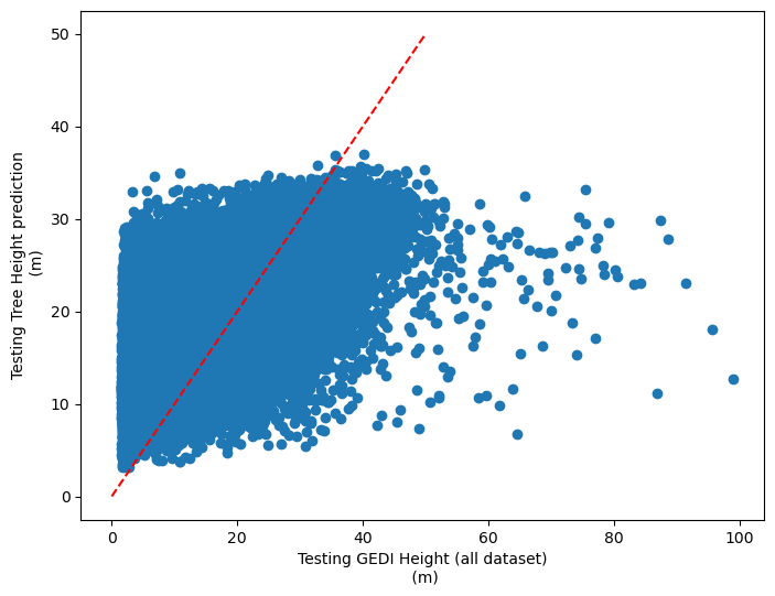
plt.rcParams["figure.figsize"] = (8,6)
plt.scatter(y_test,dic_pred['test'])
plt.xlabel('Testing GEDI Height (all dataset)\n (m)')
plt.ylabel('Testing Tree Height prediction\n (m)')
ident = [0, 50]
plt.plot(ident,ident,'r--')
[87]:
[<matplotlib.lines.Line2D at 0x712ff3e5f7d0>]

[88]:
impt = [rfReg.feature_importances_, np.std([tree.feature_importances_ for tree in rfReg.estimators_],axis=1)]
ind = np.argsort(impt[0])
[89]:
ind
[89]:
array([ 1, 13,  0,  4, 16,  6,  8, 15,  5,  2, 11,  3, 12,  9, 14,  7, 10,
       17])
[91]:
plt.rcParams["figure.figsize"] = (6,10)
plt.barh(range(len(feat)),impt[0][ind],color="b", xerr=impt[1][ind], align="center")
plt.yticks(range(len(feat)),feat[ind]);

Model Final Assesment
we can do a comparison between published model performance and ours.
Global Forest Canopy Height, 2019
[78]:
print("PEARSON CORRELATION INDEX:", pearsonr_Publication_Estimation)
PEARSON CORRELATION INDEX: 0.4527925130004339
Random Forest Model [100k GEDI subset] [fine tuning=NO] [data selection=NO]
[81]:
print("PEARSON CORRELATION COEFFINCENT:", pearsonr_all)
PEARSON CORRELATION COEFFINCENT: [0.6035710046325166, 0.506707480767017]
Random Forest Model [100k GEDI subset] [fine tuning=NO] [data selection=YES]
[83]:
print("PEARSON CORRELATION COEFFINCENT:", pearsonr_all_sel)
PEARSON CORRELATION COEFFINCENT: [0.746007848830619, 0.6125852590365624]
If we want to improve even more the selected data model, we can perform again a GridSearch hyperparameter fine tuning
pipeline = Pipeline([('rf',RandomForestRegressor())])

parameters = {
    'rf__max_features':("log2","sqrt",0.33),
    'rf__max_samples':(0.5,0.6,0.7),
    'rf__n_estimators':(500,1000),
    'rf__max_depth':(50,100,200)}
grid_search = GridSearchCV(pipeline,parameters,n_jobs=-1,cv=3,scoring='r2',verbose=1)
grid_search.fit(X_train,y_train)

grid_search.best_score_

print ('Best Training score: %0.3f' % grid_search.best_score_)
print ('Optimal parameters:')
best_par = grid_search.best_estimator_.get_params()
for par_name in sorted(parameters.keys()):
    print ('\t%s: %r' % (par_name, best_par[par_name]))

rfReg = RandomForestRegressor(n_estimators=500,max_features='sqrt',max_depth=50,max_samples=0.6,n_jobs=-1,random_state=24)
rfReg.fit(X_train, y_train);
dic_pred = {}
dic_pred['train'] = rfReg.predict(X_train)
dic_pred['test'] = rfReg.predict(X_test)
[pearsonr(dic_pred['train'],y_train)[0],pearsonr(dic_pred['test'],y_test)[0]]
Model Prediction on Raster
Predict on the raster using pyspatialml (deprecated library)
# import Global Landsat Analysis Ready Data
glad_ard_SVVI_min = "tree_height/geodata_raster/glad_ard_SVVI_min.tif"
glad_ard_SVVI_med = "tree_height/geodata_raster/glad_ard_SVVI_med.tif"
glad_ard_SVVI_max = "tree_height/geodata_raster/glad_ard_SVVI_max.tif"

# import climate data
CHELSA_bio4 = "tree_height/geodata_raster/CHELSA_bio4.tif"
CHELSA_bio18 = "tree_height/geodata_raster/CHELSA_bio18.tif"

# import soil data
BLDFIE_WeigAver = "tree_height/geodata_raster/BLDFIE_WeigAver.tif"
CECSOL_WeigAver = "tree_height/geodata_raster/CECSOL_WeigAver.tif"
ORCDRC_WeigAver = "tree_height/geodata_raster/ORCDRC_WeigAver.tif"

# import geomorphological data (DEM derived)
elev = "tree_height/geodata_raster/elev.tif"
convergence = "tree_height/geodata_raster/convergence.tif"
northness = "tree_height/geodata_raster/northness.tif"
eastness = "tree_height/geodata_raster/eastness.tif"
devmagnitude = "tree_height/geodata_raster/dev-magnitude.tif"

# import hydrographic data (from hydrography90m)
cti = "tree_height/geodata_raster/cti.tif"
outlet_dist_dw_basin = "tree_height/geodata_raster/outlet_dist_dw_basin.tif"

# import soil climate data

SBIO3_Isothermality_5_15cm = "tree_height/geodata_raster/SBIO3_Isothermality_5_15cm.tif"
SBIO4_Temperature_Seasonality_5_15cm = "tree_height/geodata_raster/SBIO4_Temperature_Seasonality_5_15cm.tif"

# import forest cover data

treecover = "tree_height/geodata_raster/treecover.tif"
from pyspatialml import Raster
predictors_rasters = [glad_ard_SVVI_min, glad_ard_SVVI_med, glad_ard_SVVI_max,
                      CHELSA_bio4,CHELSA_bio18,
                      BLDFIE_WeigAver,CECSOL_WeigAver,ORCDRC_WeigAver,
                      elev,convergence,northness,eastness,devmagnitude,cti,outlet_dist_dw_basin,
                      SBIO3_Isothermality_5_15cm,SBIO4_Temperature_Seasonality_5_15cm,treecover]

stack = Raster(predictors_rasters)
result = stack.predict(estimator=rfReg, dtype='int16', nodata=-1)
[53]:
# plot regression result
plt.rcParams["figure.figsize"] = (12,12)
result.iloc[0].cmap = "plasma"
result.plot()
plt.show()

Predict on the raster using xarray and rasterio (Full size 90m res raster prediction >12h)
import xarray as xr
import rasterio
import numpy as np
import pandas as pd
from sklearn.ensemble import RandomForestRegressor
import os

# Define paths to raster files
raster_paths = {
    'glad_ard_SVVI_min': "tree_height/geodata_raster/glad_ard_SVVI_min.tif",
    'glad_ard_SVVI_med': "tree_height/geodata_raster/glad_ard_SVVI_med.tif",
    'glad_ard_SVVI_max': "tree_height/geodata_raster/glad_ard_SVVI_max.tif",
    'CHELSA_bio4': "tree_height/geodata_raster/CHELSA_bio4.tif",
    'CHELSA_bio18': "tree_height/geodata_raster/CHELSA_bio18.tif",
    'BLDFIE_WeigAver': "tree_height/geodata_raster/BLDFIE_WeigAver.tif",
    'CECSOL_WeigAver': "tree_height/geodata_raster/CECSOL_WeigAver.tif",
    'ORCDRC_WeigAver': "tree_height/geodata_raster/ORCDRC_WeigAver.tif",
    'elev': "tree_height/geodata_raster/elev.tif",
    'convergence': "tree_height/geodata_raster/convergence.tif",
    'northness': "tree_height/geodata_raster/northness.tif",
    'eastness': "tree_height/geodata_raster/eastness.tif",
    'devmagnitude': "tree_height/geodata_raster/dev-magnitude.tif",
    'cti': "tree_height/geodata_raster/cti.tif",
    'outlet_dist_dw_basin': "tree_height/geodata_raster/outlet_dist_dw_basin.tif",
    'SBIO3_Isothermality_5_15cm': "tree_height/geodata_raster/SBIO3_Isothermality_5_15cm.tif",
    'SBIO4_Temperature_Seasonality_5_15cm': "tree_height/geodata_raster/SBIO4_Temperature_Seasonality_5_15cm.tif",
    'treecover': "tree_height/geodata_raster/treecover.tif"
}

# Load raster files into an xarray Dataset
raster_datasets = []
for name, path in raster_paths.items():
    with rasterio.open(path) as src:
        # Read raster data and convert to xarray DataArray
        data = src.read(1)  # Read the first band
        coords = {
            'y': np.linspace(src.bounds.top, src.bounds.bottom, src.height),
            'x': np.linspace(src.bounds.left, src.bounds.right, src.width)
        }
        da = xr.DataArray(data, coords=coords, dims=['y', 'x'], name=name)
        raster_datasets.append(da)

# Combine all DataArrays into a single Dataset
stack = xr.merge(raster_datasets)

# Prepare data for prediction
# Convert the stack to a 2D array where each row is a pixel and columns are features
feature_names = list(raster_paths.keys())
data_array = stack.to_array(dim='variable').transpose('y', 'x', 'variable')
data_2d = data_array.values.reshape(-1, len(feature_names))

# Create a mask for valid data (exclude pixels where any predictor is NaN)
valid_mask = ~np.any(np.isnan(data_2d), axis=1)
valid_data = data_2d[valid_mask]

# Predict tree heights for valid pixels using the trained RandomForestRegressor (rfReg)
predictions = np.full(data_2d.shape[0], -1, dtype=np.int16)  # Initialize with nodata value
predictions[valid_mask] = rfReg.predict(valid_data)

# Reshape predictions back to the original raster shape
pred_2d = predictions.reshape(data_array.shape[0], data_array.shape[1])

# Save the prediction as a new raster file
output_path = "tree_height/geodata_raster/predicted_tree_height.tif"
with rasterio.open(
    list(raster_paths.values())[0],  # Use the first raster as a template for metadata
) as src:
    profile = src.profile
    profile.update(dtype=rasterio.int16, nodata=-1)

with rasterio.open(output_path, 'w', **profile) as dst:
    dst.write(pred_2d, 1)

# Plot the result using xarray
ds_pred = xr.DataArray(pred_2d, coords={'y': stack.y, 'x': stack.x}, dims=['y', 'x'], name='predicted_height')
ds_pred.plot(cmap='plasma', figsize=(12, 12))
plt.title("Predicted Tree Height")
plt.show()
Predict on the raster using xarray and rasterio (1000x1000 UL corner tile for 90m res raster prediction)
[92]:
# Define paths to raster files
raster_paths = {
    # import Global Landsat Analysis Ready Data
    'glad_ard_SVVI_min': "tree_height/geodata_raster/glad_ard_SVVI_min.tif",
    'glad_ard_SVVI_med': "tree_height/geodata_raster/glad_ard_SVVI_med.tif",
    'glad_ard_SVVI_max': "tree_height/geodata_raster/glad_ard_SVVI_max.tif",
    # import climate data
    'CHELSA_bio4': "tree_height/geodata_raster/CHELSA_bio4.tif",
    'CHELSA_bio18': "tree_height/geodata_raster/CHELSA_bio18.tif",
    # import soil data
    'BLDFIE_WeigAver': "tree_height/geodata_raster/BLDFIE_WeigAver.tif",
    'CECSOL_WeigAver': "tree_height/geodata_raster/CECSOL_WeigAver.tif",
    'ORCDRC_WeigAver': "tree_height/geodata_raster/ORCDRC_WeigAver.tif",
    # import geomorphological data (DEM derived)
    'elev': "tree_height/geodata_raster/elev.tif",
    'convergence': "tree_height/geodata_raster/convergence.tif",
    'northness': "tree_height/geodata_raster/northness.tif",
    'eastness': "tree_height/geodata_raster/eastness.tif",
    'devmagnitude': "tree_height/geodata_raster/dev-magnitude.tif",
    # import hydrographic data (from hydrography90m)
    'cti': "tree_height/geodata_raster/cti.tif",
    'outlet_dist_dw_basin': "tree_height/geodata_raster/outlet_dist_dw_basin.tif",
    # import soil climate data
    'SBIO3_Isothermality_5_15cm': "tree_height/geodata_raster/SBIO3_Isothermality_5_15cm.tif",
    'SBIO4_Temperature_Seasonality_5_15cm': "tree_height/geodata_raster/SBIO4_Temperature_Seasonality_5_15cm.tif",
    # import forest cover data
    'treecover': "tree_height/geodata_raster/treecover.tif"
}
[93]:
import xarray as xr
import rasterio
import rasterio.windows
import numpy as np
import matplotlib.pyplot as plt
from sklearn.ensemble import RandomForestRegressor

# Define a small window (1000x1000 UL corner) to avoid high time/computation demand
window = rasterio.windows.Window(0, 0, 1000, 1000)

# Load raster files into an xarray Dataset with NoData handling
raster_datasets = []
for name, path in raster_paths.items():
    with rasterio.open(path) as src:
        # Get NoData value from raster metadata
        nodata = src.nodata if src.nodata is not None else np.nan
        # Read data within the specified window
        data = src.read(1, window=window)

        # Replace raster-specific NoData values with np.nan for consistency
        if nodata is not np.nan:
            data = np.where(data == nodata, np.nan, data)

        # Transform coordinates for the window
        transform = src.window_transform(window)
        rows, cols = np.arange(window.height), np.arange(window.width)
        xs, ys = np.meshgrid(cols, rows)
        xs_geo, ys_geo = rasterio.transform.xy(transform, ys, xs)
        x_coords = np.array(xs_geo[0])  # X coordinates for columns
        y_coords = np.array([row[0] for row in ys_geo])  # Y coordinates for rows

        # Create xarray DataArray
        da = xr.DataArray(
            data,
            coords={'y': y_coords, 'x': x_coords},
            dims=['y', 'x'],
            name=name,
            attrs={'nodata': np.nan}  # Store NoData as NaN in attributes
        )
        raster_datasets.append(da)

# Combine all DataArrays into a single Dataset
stack = xr.merge(raster_datasets)

# Prepare data for prediction
# Convert the stack to a 2D array where each row is a pixel and columns are features
feature_names = list(raster_paths.keys())
data_array = stack.to_array(dim='variable').transpose('y', 'x', 'variable')
data_2d = data_array.values.reshape(-1, len(feature_names))

# Create a mask for valid data (exclude pixels where any predictor is NaN)
valid_mask = ~np.any(np.isnan(data_2d), axis=1)
valid_data = data_2d[valid_mask]

# Predict tree heights for valid pixels using the trained RandomForestRegressor
predictions = np.full(data_2d.shape[0], -1, dtype=np.int16)  # Initialize with NoData value (-1)
if valid_data.size > 0:  # Ensure there is valid data to predict
    predictions[valid_mask] = rfReg.predict(valid_data).astype(np.int16)
else:
    print("Warning: No valid data (non-NoData pixels) available for prediction.")

# Reshape predictions back to the original raster shape
pred_2d = predictions.reshape(data_array.shape[0], data_array.shape[1])

# Save the prediction as a new raster file
output_path = "tree_height/geodata_raster/predicted_tree_height_light.tif"
with rasterio.open(list(raster_paths.values())[0]) as src:
    profile = src.profile
    profile.update(
        dtype=rasterio.int16,
        nodata=-1,  # Explicitly set NoData value
        width=window.width,
        height=window.height,
        transform=src.window_transform(window)
    )

with rasterio.open(output_path, 'w', **profile) as dst:
    dst.write(pred_2d, 1)

# Plot the result using xarray with NoData masking
ds_pred = xr.DataArray(
    pred_2d,
    coords={'y': stack.y, 'x': stack.x},
    dims=['y', 'x'],
    name='predicted_tree_height',
    attrs={'nodata': -1}
)

# Mask NoData values (-1) for visualization
ds_pred_masked = ds_pred.where(ds_pred != -1)

# Plot with a colorbar and appropriate scaling for tree heights
plt.figure(figsize=(15, 15))
ds_pred_masked.plot(cmap='viridis', cbar_kwargs={'label': 'Tree Height (m)'})
plt.title("Predicted Tree Height (1000x1000px, NoData masked)")
plt.xlabel("X (geographic)")
plt.ylabel("Y (geographic)")
plt.show()
