{
"cells": [
{
"cell_type": "markdown",
"id": "06d8b892-a347-470b-af38-1f4949cf8144",
"metadata": {
"id": "06d8b892-a347-470b-af38-1f4949cf8144"
},
"source": [
"# Python data analysis\n",
"\n",
"Saverio Mancino\n",
"\n",
"--------------\n"
]
},
{
"cell_type": "markdown",
"id": "3a2dc50e-db6d-4521-a6d6-57c5dce1d0c1",
"metadata": {},
"source": [
"## Open the notebook lesson\n",
"\n",
"Open the lesson using the CL\n",
"\n",
" cd /media/sf_LVM_shared/my_SE_data/exercise\n",
" jupyter-lab Python_data_analysis_SM.ipynb\n"
]
},
{
"cell_type": "markdown",
"id": "289b53c1-511f-4139-b26b-7629ad651bf2",
"metadata": {
"id": "289b53c1-511f-4139-b26b-7629ad651bf2"
},
"source": [
"## Lesson Overview\n",
"\n",
"This lesson is designed to provide a thorough understanding of data handling using Python.\n",
"You will learn how to work with numerical data using Numpy and handle tabular data using Pandas.\n",
"The lesson includes:\n",
"\n",
"- Detailed explanations of key concepts;\n",
"- Python code examples in executable cells;\n",
"- Exercise boxes with challenges to test your understanding.\n"
]
},
{
"cell_type": "markdown",
"id": "94633668-3abb-460a-9ba8-dff4cdcd8d37",
"metadata": {
"id": "94633668-3abb-460a-9ba8-dff4cdcd8d37"
},
"source": [
"## Objectives\n",
"\n",
"By the end of this lesson, you should be able to:\n",
"\n",
"- Knowing the Jupyter enviroment for python programming;\n",
"- Understand the basics of Numpy for numerical operations\n",
"- Create and manipulate Numpy arrays\n",
"- Understand the fundamentals of Pandas, including Series and DataFrames\n",
"- Import, clean, and analyze data using Pandas\n",
"- Apply advanced data handling techniques such as grouping, merging, and pivoting\n",
"- Solve practical exercises to reinforce your learning"
]
},
{
"cell_type": "markdown",
"id": "64e13af6-a1ce-497a-b274-d35d42a7f276",
"metadata": {
"id": "64e13af6-a1ce-497a-b274-d35d42a7f276"
},
"source": [
"------------------------\n",
"\n",
"## Table of Contents\n",
"\n",
"1. [Jupyter Environment for Python Programming](#1)\n",
"2. [GitHub and Code Repository Versioning Systems](#2)\n",
"3. [Introduction](#3)\n",
"4. [Numpy Basics](#4)\n",
"5. [Pandas Basics](#5)\n",
"7. [Exercises](#6)\n",
"\n",
"\n",
"------------"
]
},
{
"cell_type": "markdown",
"id": "bca33ffa-c138-4ea7-97f6-f6b1d9a59d50",
"metadata": {
"id": "bca33ffa-c138-4ea7-97f6-f6b1d9a59d50"
},
"source": [
"## 1 - Environments for Python Programming\n",
"\n",
"### Python Kernel\n",
"The Python kernel is the component that executes your Python code within a Jupyter Notebook. When you run a cell, the kernel processes the code and returns the output. Also, the kernel maintains the state of your session, including variable definitions, imported modules, and function declarations. This means that cells can depend on code executed in previous cells.\n",
"Infact, Jupyter provides also the options to restart or interrupt the kernel.\n",
"This is useful for clearing the workspace or stopping long-running processes without having to close the entire notebook.\n",
"\n",
"### Jupyter Notebook\n",
"Jupyter is an open-source, locally managed, web coding application for project development.\n",
"\n",
"\n",
"\n",
"A Jupyter notebook has two components: a front-end web page and a back-end kernel. The front-end web page allows data scientists to enter programming code or text into rectangular ‘cells’. The browser then passes the code to the back-end kernel, which executes it and returns the results.\n",
"Its characterised by:\n",
"\n",
"- **Interactive Computing:**\\\n",
"Jupyter Notebooks let you run code in an interactive, cell-by-cell manner. This enables iterative development and immediate feedback, which is especially useful when testing new ideas or debugging.\n",
"\n",
"- **Integrated Documentation:**\\\n",
"Combine rich text (using Markdown), live code, and visualizations in a single document. This integration supports reproducible research and thorough documentation of your data analysis workflow.\n",
"\n",
"- **Multi-Language Support:**\\\n",
"Although originally designed for Python and Bash, Jupyter supports many programming languages (e.g., R, Julia) through the use of kernels. This flexibility allows you to work with multiple languages in one environment.\n",
"\n",
"- **Ease of Sharing:**\\\n",
"Notebooks can be easily shared and converted into different formats (HTML, PDF, slides), making it simple to disseminate your work among colleagues or publish it online.\n",
"\n",
"### Google Colab\n",
"\n",
"Google Colab is a cloud-based Jupyter Notebook environment developed by Google.\n",
"\n",
"\n",
"\n",
"It allows users to write and execute Python code in an interactive notebook format without requiring any local setup.\n",
"Google Colab is particularly useful for Python beginners, researchers, and data scientists who want a hassle-free environment for coding, data analysis, and machine learning experiments.\n",
"\n",
"- **No Installation Required:**\\\n",
"Colab runs entirely in the cloud, so there's no need to install Python, Jupyter, or any dependencies.\n",
"\n",
"- **Free GPU and TPU Access:**\\\n",
" Google provides free access to GPUs and TPUs, making it a great choice for machine learning and data science projects.\n",
"\n",
"- **Integration with Google Drive:**\\\n",
"You can save and load files directly from Google Drive, making it easy to store and share your work.\n",
"\n",
"- **Collaboration:**\\\n",
"Multiple users can edit and run the same notebook simultaneously, similar to Google Docs.\n",
"\n",
"- **Pre-installed Libraries:**\\\n",
"Colab comes already with popular Python libraries such as NumPy, Pandas, TensorFlow, and Matplotlib pre-installed.\n",
"\n",
"#### Using Google Colab:\n",
"\n",
"- **Access Colab:**\\\n",
"Open Google Colab in your browser.\n",
"- **Create a New Notebook:**\\\n",
"Click on \"New Notebook\" to start coding in Python.\n",
"- **Upload Files:**\\\n",
"Use files.upload() from google.colab to upload datasets.\n"
]
},
{
"cell_type": "markdown",
"id": "381e5932-914c-4316-bf2e-c0dad02e60b4",
"metadata": {
"id": "381e5932-914c-4316-bf2e-c0dad02e60b4"
},
"source": [
"## 2 - GitHub and Code Repository Versioning Systems\n",
"\n",
"In modern software development and data science projects, version control systems are essential for maintaining code integrity, tracking changes, and enabling collaboration.\n",
"This subchapter provides an overview of GitHub, along with other code repository and versioning systems commonly used in the field.\n",
"\n",
"### What is Version Control?\n",
"\n",
"Version control is a system that records changes to a file or set of files over time. This allows you to:\n",
"- **Revert to Previous Versions:** Easily roll back to earlier iterations if errors or issues arise.\n",
"- **Collaborate Efficiently:** Multiple developers can work on the same project simultaneously without overwriting each other's work.\n",
"- **Track Changes:** Maintain a detailed history of modifications, including who made the changes and why.\n",
"\n",
"### Git and Its Ecosystem\n",
"\n",
"- **Git:** \n",
" Git is a distributed version control system that lets every developer maintain a complete local copy of the project history. Its branching and merging features facilitate experimentation and efficient collaboration.\n",
"- **Repositories:** \n",
" A repository (or repo) is the storage space for your project's files along with their version history. Repositories can be local (on your machine) or hosted remotely.\n",
"\n",
"### GitHub\n",
"\n",
"\n",
"\n",
"\n",
"- **What is GitHub?** \n",
" [GitHub](https://github.com/) is a web-based platform built around Git. It provides an intuitive interface for hosting, managing, and collaborating on Git repositories.\n",
"- **Key Features:**\n",
" - **Pull Requests:** \n",
" Enable developers to propose changes, review code collaboratively, and merge updates into the main project after thorough discussion.\n",
" - **Issue Tracking & Project Management:** \n",
" Built-in tools to manage bugs, track feature requests, and plan project workflows.\n",
" - **Continuous Integration (CI):** \n",
" Integration with CI/CD tools automates testing and deployment, ensuring that code changes meet quality standards before they are merged.\n",
" - **Community & Open Source:** \n",
" GitHub hosts millions of open-source projects, making it a vibrant community for sharing and contributing to software development.\n",
"\n",
"There are many other popular platforms like GitLab, Bitbucket etc., wich offers similar functionalities to GitHub with a different emphasis on other features.\n"
]
},
{
"cell_type": "markdown",
"id": "36eaa513-4f24-4d15-8222-fd3be501ad60",
"metadata": {
"id": "36eaa513-4f24-4d15-8222-fd3be501ad60"
},
"source": [
"## 3 - Introduction\n",
"\n",
"In today’s world, data is at the heart of decision-making across industries: from scientific research to finance, healthcare and social media.\n",
"This lesson is designed to equip you with essential skills in data handling using Python, focusing on two of its most powerful libraries: Numpy and Pandas.\n",
"\n",
"### The Importance of Data Handling\n",
"\n",
"With the exponential growth in the volume of data generated every day, having robust tools and methodologies to handle, clean, and analyze data is more crucial than ever.\n",
"Thats why an effective data management and analysis can uncover insights that drive strategic decisions. Expecially in conducting scientific research the ability to interpret data accurately is invaluable.\n",
"Automated data handling tools use is spreading to minimizes human error and increases the speed of data processing.\n",
"By leveraging Python’s libraries, you can streamline tasks that would otherwise be time-consuming if done manually.\n",
"Its important to be comfortable with manipulating data in Python but also prepared to tackle more complex data challenges, in this sense mastering Numpy and Pandas lays the groundwork for more advanced topics in data science, including machine learning, statistical analysis, and data visualization.\n",
"\n",
"### Bash vs Python: Memory Usage and Use Cases\n",
"\n",
"Bash and Python are two powerful tools for data processing, but they have different strengths and weaknesses.\\\n",
"\n",
"Bash is efficient for:\n",
"- Handling large text files (e.g., `awk`, `sed`, `grep`);\n",
"- Processing streams without loading data into memory;\n",
"- Automating workflows and integrating different programs;\n",
"- Dealing with high-latency remote server/cluster.\n",
"\n",
"However, Bash has limitations in:\n",
"- Complex data structures (e.g., arrays, dictionaries);\n",
"- Advanced mathematical operations;\n",
"- Readability and debugging;\n",
"\n",
"### When to Use Python\n",
"\n",
"Python language is preferred for:\n",
"- Complex data manipulations (e.g., NumPy, Pandas);\n",
"- Machine learning and data analysis;\n",
"- Scripts requiring structured programming and logic;\n",
"\n",
"However, Python differently from bash, loads all data into memory, which can be inefficient for very large files compared to streaming in Bash.\n",
"\n",
"### Language Snippets\n",
"\n",
"One of the most powerfull tecnique consinst in using small code snippets of Python in Bash or vice versa.\n",
"Switching code language with snippets it's like switching gears while driving a car.\n",
"\n",
"- Bash as the first gear: Ideal for quick tasks, file manipulation, and streaming large datasets without loading them entirely.\n",
"- Python as the fifth gear: Powerfull, best for complex calculations, structured data manipulations, and advanced analysis and modeling.\n",
"\n",
"Mastering the switch between Bash and Python snippets can significantly optimize workflows and memory usage.\n",
"\n",
"### What You Will Learn\n",
"\n",
"- **Fundamentals of Numpy:** Learn how to create and manipulate multi-dimensional arrays, perform vectorized operations, and understand how these methods offer significant performance improvements over traditional Python loops.\n",
"- **Pandas for Structured Data:** Discover how to create and manage data using Pandas DataFrames and Series. You’ll learn methods for cleaning, transforming, and summarizing data, enabling you to work efficiently with large datasets.\n",
"- **Advanced Techniques:** Delve into more sophisticated operations such as merging datasets, grouping data for aggregate analysis, and creating pivot tables to reorganize and summarize complex data structures.\n",
"- **Hands-On Practice:** This lesson incorporates practical exercises and code examples, giving you the opportunity to apply theoretical knowledge to real-world data scenarios. Each exercise is designed to reinforce your learning and build your confidence in using Python for data handling.\n"
]
},
{
"cell_type": "markdown",
"id": "b1ff46bd-cfe2-4704-bb77-868ca3ee8fc4",
"metadata": {},
"source": [
"## Data Retrieving\n",
"\n",
"Before proceeding with the lesson, run this code to download to the virtual machine the files that will be used in these python lessons"
]
},
{
"cell_type": "code",
"execution_count": null,
"id": "8a8347f3-11ab-4709-93e6-ea133b959e11",
"metadata": {},
"outputs": [],
"source": [
"!pip install gdown"
]
},
{
"cell_type": "code",
"execution_count": null,
"id": "d5bcee5c-a39d-4edb-9b2e-e8e192641397",
"metadata": {},
"outputs": [],
"source": [
"import gdown\n",
"!mkdir -p /media/sf_LVM_shared/my_SE_data/exercise/files\n",
"file_url = 'https://drive.google.com/uc?export=download&id=1J54Xpk-qHnz7yuIYSqOgVQy6_QpYhLVv'\n",
"output_path = '/media/sf_LVM_shared/my_SE_data/exercise/files/file.zip'\n",
"gdown.download(file_url, output_path, quiet=False)\n",
"!unzip /media/sf_LVM_shared/my_SE_data/exercise/files/file.zip -d /media/sf_LVM_shared/my_SE_data/exercise/files\n",
"!rm /media/sf_LVM_shared/my_SE_data/exercise/files/file.zip"
]
},
{
"cell_type": "markdown",
"id": "0adca23a-f42d-49b2-a69f-26f312769c90",
"metadata": {
"id": "0adca23a-f42d-49b2-a69f-26f312769c90"
},
"source": [
"## 4 - Numpy Basics\n",
"\n",
"\n",
"\n",
"Numpy is a powerful Python library specifically designed for numerical computations and data manipulations.\\\n",
"We will learn how to create and manipulate numpy arrays, which are useful matrix-like structures for holding large amounts of data\n",
"We will cover:\n",
"\n",
"- Creating Numpy arrays;\n",
"- Basic arithmetic and vectorized operations;\n",
"- Indexing, slicing, and reshaping arrays;"
]
},
{
"cell_type": "markdown",
"id": "bf097fea-9291-4d10-8373-3604e56d8d9b",
"metadata": {
"id": "bf097fea-9291-4d10-8373-3604e56d8d9b"
},
"source": [
"In order to be able to use numpy we need to import the numpy library using ```import```.\\\n",
"Imports in Python avoid us typing numpy every time for using some functions, providing an alias us ```as``` instead.\\\n",
"It's commonly nicknamed ```numpy as np```"
]
},
{
"cell_type": "code",
"execution_count": 1,
"id": "979da7ee-d7a9-473c-bac5-857661065942",
"metadata": {
"id": "979da7ee-d7a9-473c-bac5-857661065942"
},
"outputs": [],
"source": [
"# Importing necessary libraries\n",
"import numpy as np\n",
"import pandas as pd\n",
"from PIL import Image"
]
},
{
"cell_type": "markdown",
"id": "cffc89d2-90be-41ff-8638-856fb9b55145",
"metadata": {},
"source": [
"If `numpy` import doesn't work properly the following bash lines should be run"
]
},
{
"cell_type": "code",
"execution_count": 5,
"id": "42d5e253-52be-45f9-ba10-2408fab06ea0",
"metadata": {},
"outputs": [],
"source": [
"# !pip show numpy pandas | grep Version:"
]
},
{
"cell_type": "code",
"execution_count": 6,
"id": "5eae79de-cf0a-4584-a736-c9e5ac6c2fc5",
"metadata": {},
"outputs": [],
"source": [
"# !pip uninstall -y numpy"
]
},
{
"cell_type": "code",
"execution_count": 7,
"id": "df8a844e-9681-4393-bca2-db58257419a6",
"metadata": {},
"outputs": [],
"source": [
"# !pip install numpy==1.23.0"
]
},
{
"cell_type": "markdown",
"id": "ca745eaa-ca05-4630-a978-edb5591d305b",
"metadata": {
"id": "ca745eaa-ca05-4630-a978-edb5591d305b"
},
"source": [
"Now, we have access to all the functions available in numpy by typing `np.name_of_function`.\\"
]
},
{
"cell_type": "markdown",
"id": "70cc9d64-e66e-4795-b23a-15d47dc7743b",
"metadata": {
"id": "70cc9d64-e66e-4795-b23a-15d47dc7743b"
},
"source": [
"### Arrays\n",
"\n",
"An **array** is a data structure that stores multiple values in a single variable. Unlike individual variables that hold a single piece of data, arrays allow you to work with collections of data efficiently.\\\n",
"Arrays are commonly used in programming and data analysis because they provide a structured way to store and manipulate large datasets.\\\n",
"Arrays are used to reducing memory overhead compared to using multiple separate variables, providing optimized access and modification methods, which are significantly faster than working with regular Python lists, especially for large datasets.\\\n",
"Futhermore, arrays support vectorized operations, meaning you can perform arithmetic operations on entire arrays at once without using loops.\n",
"\n",
"#### Arrays in Python\n",
"\n",
"In Python, arrays can be implemented in different ways:\n",
"\n",
"- **Lists:** Python’s built-in lists can store different data types but are not optimized for numerical computations.\n",
"- **NumPy Arrays:** NumPy provides specialized arrays that are more memory-efficient and allow fast mathematical operations.\n",
"\n"
]
},
{
"cell_type": "markdown",
"id": "b3c0bec8-b148-4cf1-ab0e-bd7e7d4d849f",
"metadata": {
"id": "b3c0bec8-b148-4cf1-ab0e-bd7e7d4d849f"
},
"source": [
"### Numpy arrays\n",
"\n",
"One of numpy’s core concepts is the array. They can hold multi-dimensional data. To declare a numpy array explicity we do ```np.array([])```.\\\n",
"For instance thats and example of a 1D array."
]
},
{
"cell_type": "code",
"execution_count": 8,
"id": "18fd8fa4-e3ca-41c3-931f-937582ba3741",
"metadata": {
"colab": {
"base_uri": "https://localhost:8080/"
},
"id": "18fd8fa4-e3ca-41c3-931f-937582ba3741",
"outputId": "51d0133d-03ee-4ac9-81f9-2f328a84a0f2"
},
"outputs": [
{
"data": {
"text/plain": [
"array([1, 2, 3, 4, 5, 6, 7, 8, 9])"
]
},
"execution_count": 8,
"metadata": {},
"output_type": "execute_result"
}
],
"source": [
"np.array([1,2,3,4,5,6,7,8,9])"
]
},
{
"cell_type": "markdown",
"id": "f563b312-f373-4999-a58f-927ce4426d9c",
"metadata": {
"id": "f563b312-f373-4999-a58f-927ce4426d9c"
},
"source": [
"Most of the functions and operations defined in numpy can be applied to arrays.\\\n",
"For example, with the previous add operation:"
]
},
{
"cell_type": "code",
"execution_count": 9,
"id": "018258ec-f7bb-45e5-b9ba-7e70b37cb712",
"metadata": {
"colab": {
"base_uri": "https://localhost:8080/"
},
"id": "018258ec-f7bb-45e5-b9ba-7e70b37cb712",
"outputId": "40b218ff-7bd1-4044-ef4e-04330035cfc6"
},
"outputs": [
{
"data": {
"text/plain": [
"array([ 4, 6, 8, 10])"
]
},
"execution_count": 9,
"metadata": {},
"output_type": "execute_result"
}
],
"source": [
"arr1 = np.array([1,2,3,4])\n",
"arr2 = np.array([3,4,5,6])\n",
"\n",
"np.add(arr1, arr2)"
]
},
{
"cell_type": "markdown",
"id": "6a7bcbec-cbc5-42e8-b8e2-4f66de23c52a",
"metadata": {
"id": "6a7bcbec-cbc5-42e8-b8e2-4f66de23c52a"
},
"source": [
"We can also add arrays using the following convenient notation:"
]
},
{
"cell_type": "code",
"execution_count": 10,
"id": "e472ce7e-2e90-41c6-a37c-039cd6c36217",
"metadata": {
"colab": {
"base_uri": "https://localhost:8080/"
},
"id": "e472ce7e-2e90-41c6-a37c-039cd6c36217",
"outputId": "c187dd9e-71fd-4fd2-e131-1a2db75b26b2"
},
"outputs": [
{
"data": {
"text/plain": [
"array([ 4, 6, 8, 10])"
]
},
"execution_count": 10,
"metadata": {},
"output_type": "execute_result"
}
],
"source": [
"arr1 + arr2"
]
},
{
"cell_type": "markdown",
"id": "5b9169a5-11d4-4dc3-8d91-c66597bbc353",
"metadata": {
"id": "5b9169a5-11d4-4dc3-8d91-c66597bbc353"
},
"source": [
"Arrays can be sliced and diced.\\\n",
"We can get subsets of the arrays using the indexing notation which is ```[ start : end : stride ]```.\\\n",
"Let’s see what this means:"
]
},
{
"cell_type": "code",
"execution_count": 11,
"id": "62e7d4ba-710f-4688-8fc4-fc602f35578e",
"metadata": {
"colab": {
"base_uri": "https://localhost:8080/"
},
"id": "62e7d4ba-710f-4688-8fc4-fc602f35578e",
"outputId": "3bc3e611-a55c-4b45-f71f-05f57c57efd6"
},
"outputs": [
{
"name": "stdout",
"output_type": "stream",
"text": [
"5\n",
"[ 5 6 7 8 9 10 11 12 13 14 15]\n",
"[0 1 2 3 4]\n",
"[ 0 2 4 6 8 10 12 14]\n"
]
}
],
"source": [
"arr = np.array([0,1,2,3,4,5,6,7,8,9,10,11,12,13,14,15])\n",
"\n",
"print(arr[5]) # show 5° position\n",
"print(arr[5:]) # start from 5° position\n",
"print(arr[:5]) # end on 5° position\n",
"print(arr[::2]) # Reading step set as 2"
]
},
{
"cell_type": "markdown",
"id": "e6f73bea-345f-434b-a6ee-729eca6d8e43",
"metadata": {
"id": "e6f73bea-345f-434b-a6ee-729eca6d8e43"
},
"source": [
"**Numpy indexes start on 0**, the same convention used in Python lists. But indexes can also be negative, meaning that you start counting by the end.\\\n",
"For example, to select the last 2 elements in an array we can do:"
]
},
{
"cell_type": "code",
"execution_count": 12,
"id": "4650c0db-0298-4ae6-9b02-ff4207351be4",
"metadata": {
"colab": {
"base_uri": "https://localhost:8080/"
},
"id": "4650c0db-0298-4ae6-9b02-ff4207351be4",
"outputId": "119a9222-d003-47ea-fe00-8d1651707d4e"
},
"outputs": [
{
"data": {
"text/plain": [
"array([14, 15])"
]
},
"execution_count": 12,
"metadata": {},
"output_type": "execute_result"
}
],
"source": [
"arr = np.array([0,1,2,3,4,5,6,7,8,9,10,11,12,13,14,15])\n",
"\n",
"arr[-2:] # show the first 2 elements from the last position"
]
},
{
"cell_type": "markdown",
"id": "a29c427e-751a-4bcd-92d3-b7ae65bf7d84",
"metadata": {
"id": "a29c427e-751a-4bcd-92d3-b7ae65bf7d84"
},
"source": [
"In this way we can freely access and easly manipulate the information contained in the arrays.\\\n",
"For example:"
]
},
{
"cell_type": "code",
"execution_count": 13,
"id": "aa025fd2-73e1-4793-b664-ae756a1235f1",
"metadata": {
"colab": {
"base_uri": "https://localhost:8080/"
},
"id": "aa025fd2-73e1-4793-b664-ae756a1235f1",
"outputId": "fc7aad3b-556b-4621-877e-34e1d8b7db81"
},
"outputs": [
{
"name": "stdout",
"output_type": "stream",
"text": [
"Original array: [1 2 3 4 5]\n",
"After adding one: [2 3 4 5 6]\n",
"Slice (indexes 1 to 3): [2 3 4]\n"
]
}
],
"source": [
"# We can create a Numpy array\n",
"a = np.array([1, 2, 3, 4, 5])\n",
"print('Original array:', a)\n",
"\n",
"# We can manipulate it with some basic arithmetic operations\n",
"# adding elements\n",
"b = a + 1\n",
"print('After adding one:', b)\n",
"\n",
"# or subtracting elements\n",
"slice_a = a[1:4]\n",
"print('Slice (indexes 1 to 3):', slice_a)"
]
},
{
"cell_type": "markdown",
"id": "a29b166f-de12-4ac1-bf38-4ac2fc124504",
"metadata": {
"id": "a29b166f-de12-4ac1-bf38-4ac2fc124504"
},
"source": [
"Numpy arrays can have multiple dimensions.\\\n",
"Dimensions are indicated using nested square brackets ```[ ]```.\\\n",
"The convention in numpy is that the outer ```[ ]``` represent the first dimension and the innermost ```[ ]``` contains the last dimension.\n",
"\n",
"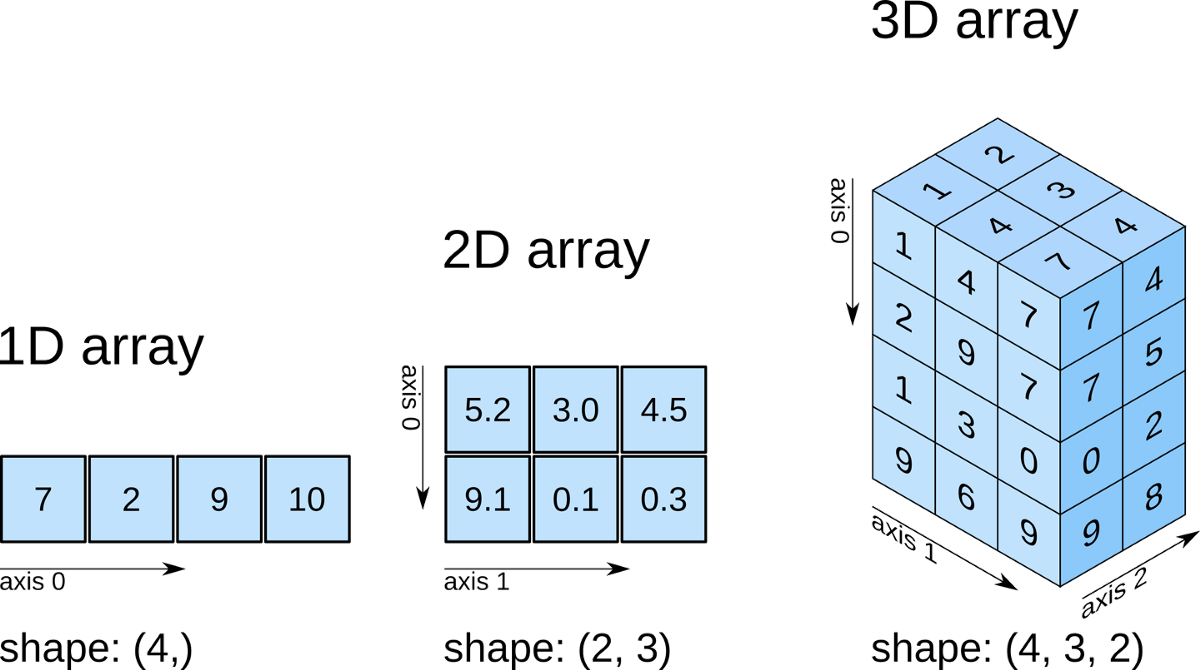\n",
"\n",
"Now we declare a 2D array with shape (1, 9).\n",
"In this case, the nested (double) square brackets ```[[ ]]``` indicates the array is 2-dimensional."
]
},
{
"cell_type": "code",
"execution_count": 14,
"id": "0c00bce7-aa73-4aa9-b22d-209781b750cc",
"metadata": {
"colab": {
"base_uri": "https://localhost:8080/"
},
"id": "0c00bce7-aa73-4aa9-b22d-209781b750cc",
"outputId": "acf25dfe-f752-46d9-9d74-0c1c345dec67"
},
"outputs": [
{
"data": {
"text/plain": [
"array([[1, 2, 3, 4, 5, 6, 7, 8, 9]])"
]
},
"execution_count": 14,
"metadata": {},
"output_type": "execute_result"
}
],
"source": [
"np.array([[1,2,3,4,5,6,7,8,9]])"
]
},
{
"cell_type": "markdown",
"id": "9edd8f75-5d8e-4ff7-8802-b098de763080",
"metadata": {
"id": "9edd8f75-5d8e-4ff7-8802-b098de763080"
},
"source": [
"To visualise the shape (dimensions) of a numpy array we can add the suffix `.shape` to an array expression or variable containing a numpy array."
]
},
{
"cell_type": "code",
"execution_count": 15,
"id": "66c93ff0-9ac0-424a-ad00-7a445355a837",
"metadata": {
"colab": {
"base_uri": "https://localhost:8080/"
},
"id": "66c93ff0-9ac0-424a-ad00-7a445355a837",
"outputId": "4c1ac91f-87aa-4eba-8141-e1bfa3ec7224"
},
"outputs": [
{
"name": "stdout",
"output_type": "stream",
"text": [
"arr1 shape: (9,) arr2 shape: (1, 9) arr3 shape: (9, 1) arr4 shape: (3,) \n"
]
}
],
"source": [
"arr1 = np.array([1,2,3,4,5,6,7,8,9]) # 1D array\n",
"arr2 = np.array([[1,2,3,4,5,6,7,8,9]]) # 2D array\n",
"arr3 = np.array([[1],[2],[3],[4],[5],[6],[7],[8],[9]]) # 2D array\n",
"arr4 = np.array([1,2,3]) # 1D array\n",
"\n",
"print(f\"\\\n",
"arr1 shape: {arr1.shape} \\\n",
"arr2 shape: {arr2.shape} \\\n",
"arr3 shape: {arr3.shape} \\\n",
"arr4 shape: {arr4.shape} \\\n",
"\")"
]
},
{
"cell_type": "markdown",
"id": "3efcd81e-79c5-4922-a4ad-687775baff7a",
"metadata": {
"id": "3efcd81e-79c5-4922-a4ad-687775baff7a"
},
"source": [
"Numpy arrays can contain numerical values of different types.\\\n",
"These types can be divided in these groups:\n",
"\n",
"|Unsigned Integers||\n",
"|:---:|:---:|\n",
"|bits|alias|\n",
"| 8 bits | uint8 |\n",
"| 16 bits | uint16 |\n",
"| 32 bits | uint32 |\n",
"| 64 bits | uint64 |\n",
"\n",
"|Signed Integers||\n",
"|:---:|:---:|\n",
"|bits|alias|\n",
"|8 bits | int8 |\n",
"| 16 bits | int16 |\n",
"| 32 bits | int32 |\n",
"| 64 bits | int64\n",
"\n",
"|Floats||\n",
"|:---:|:---:|\n",
"|bits|alias|\n",
"|32 bits| float32|\n",
"|64 bits| float64|"
]
},
{
"cell_type": "markdown",
"id": "3b1c5fe1-24a4-4d1d-b358-676cb8c30873",
"metadata": {
"id": "3b1c5fe1-24a4-4d1d-b358-676cb8c30873"
},
"source": [
"We can look up the type of an array by using the ```.dtype``` suffix."
]
},
{
"cell_type": "code",
"execution_count": 12,
"id": "eecf479b-607a-4313-8912-78228a8496fe",
"metadata": {
"colab": {
"base_uri": "https://localhost:8080/"
},
"id": "eecf479b-607a-4313-8912-78228a8496fe",
"outputId": "6046f258-1693-47db-c1c9-3668b8b89973"
},
"outputs": [
{
"name": "stdout",
"output_type": "stream",
"text": [
"shape: (10, 10, 10)\n",
"type: float64\n",
"weight: 7.81 kB\n",
"type: bool\n",
"weight: 0.98 kB\n"
]
}
],
"source": [
"arr = np.ones((10,10,10))\n",
"\n",
"# In this way we created a 10x10x10 matrix populated only by '1'\n",
"# arr\n",
"\n",
"print (f\"shape: {arr.shape}\")\n",
"print (f\"type: {arr.dtype}\")\n",
"print (f\"weight: {round((arr.nbytes / 1024),2)} kB\")\n",
"arr_bool = arr.astype(bool)\n",
"print (f\"type: {arr_bool.dtype}\")\n",
"print (f\"weight: {round((arr_bool.nbytes / 1024),2)} kB\")"
]
},
{
"cell_type": "markdown",
"id": "7fb6a10f-851c-48c2-ae06-4afe59b09d9c",
"metadata": {
"id": "7fb6a10f-851c-48c2-ae06-4afe59b09d9c"
},
"source": [
"Numpy arrays normally store numeric values but they can also contain boolean values, `bool`.\\\n",
"Boolean is a data type that can have two possible values: `True` or `False`.\\\n",
"For example:"
]
},
{
"cell_type": "code",
"execution_count": 9,
"id": "aded8ce6-b2e6-4e3e-b9c4-35c24c3e0af0",
"metadata": {
"colab": {
"base_uri": "https://localhost:8080/"
},
"id": "aded8ce6-b2e6-4e3e-b9c4-35c24c3e0af0",
"outputId": "72adf8fa-793d-4b02-cd3e-eaa0767af189"
},
"outputs": [
{
"name": "stdout",
"output_type": "stream",
"text": [
"bool array: [ True False True]\n",
"array shape: (3,)\n",
"array type: bool\n"
]
}
],
"source": [
"arr = np.array([True, False, True]) # declaring a 1D bool array\n",
"\n",
"print(\"bool array:\", arr)\n",
"print(\"array shape: \", arr.shape)\n",
"print(\"array type: \", arr.dtype)"
]
},
{
"cell_type": "markdown",
"id": "893e6dfc-a9bb-4174-8fa4-62b5104df29e",
"metadata": {
"id": "893e6dfc-a9bb-4174-8fa4-62b5104df29e"
},
"source": [
"### Numpy Operations\n",
"\n",
"- **Arithmetic Operations:** Numpy supports element-wise operations, allowing you to add, subtract, multiply, or divide arrays directly.\n",
"- **Slicing and Indexing:** Similar to Python lists, arrays can be sliced using the `[start:stop]` syntax.\n",
"\n",
"Let's explore further operations such as reshaping and broadcasting."
]
},
{
"cell_type": "markdown",
"id": "57af1308-6e24-4860-b636-c5953f1fcc7a",
"metadata": {
"id": "57af1308-6e24-4860-b636-c5953f1fcc7a"
},
"source": [
"We can operate with boolean arrays using the numpy functions for performing logical operations such as `and` and `or`.\\\n",
"These operations are conveniently offered by numpy with the symbols `*` (`and`), and `+` (`or`).\n",
"\n",
"*Note: Here the `*` and `+` symbols are not performing multiplication and addition as with numerical arrays.\\\n",
"Numpy detects the type of the arrays involved in the operation and changes the behaviour of these operators.*"
]
},
{
"cell_type": "code",
"execution_count": 18,
"id": "98466567-a8ee-4f85-9369-ceeb0dfc6a7d",
"metadata": {
"colab": {
"base_uri": "https://localhost:8080/"
},
"id": "98466567-a8ee-4f85-9369-ceeb0dfc6a7d",
"outputId": "a3ebc592-c777-434f-df7d-9f0d525404a8"
},
"outputs": [
{
"name": "stdout",
"output_type": "stream",
"text": [
"AND operator\n",
"[ True False False False]\n",
"[ True False False False]\n",
"OR operator\n",
"[ True True True False]\n",
"[ True True True False]\n"
]
}
],
"source": [
"arr1 = np.array([True, True, False, False])\n",
"arr2 = np.array([True, False, True, False])\n",
"\n",
"# two way to use AND operator\n",
"print (\"AND operator\")\n",
"print(np.logical_and(arr1, arr2))\n",
"print(arr1 * arr2)\n",
"\n",
"# two way to use OR operator\n",
"print (\"OR operator\")\n",
"print(np.logical_or(arr1, arr2))\n",
"print(arr1 + arr2)"
]
},
{
"cell_type": "markdown",
"id": "0f0d30a6-d701-4781-a57f-03662ba099f3",
"metadata": {
"id": "0f0d30a6-d701-4781-a57f-03662ba099f3"
},
"source": [
"Boolean arrays are often the result of comparing a numerical arrays with certain values.\\\n",
"This is sometimes useful to detect values that are equal, below or above a number in a numpy array.\\\n",
"For example, if we want to know which values in an array are equal to 1, and the values that are greater than 2 we can do:"
]
},
{
"cell_type": "code",
"execution_count": 11,
"id": "5c2dd374-2a0b-4d9a-af4b-4bddda510c0a",
"metadata": {
"colab": {
"base_uri": "https://localhost:8080/"
},
"id": "5c2dd374-2a0b-4d9a-af4b-4bddda510c0a",
"outputId": "a4c475aa-2774-4a39-b1dc-5d5881effb3e"
},
"outputs": [
{
"name": "stdout",
"output_type": "stream",
"text": [
"[ True False False True False False True False False True]\n",
"[False True True False True True False True True False]\n"
]
}
],
"source": [
"arr = np.array([1, 3, 5, 1, 6, 3, 1, 5, 7, 1])\n",
"\n",
"print(arr == 1)\n",
"print(arr > 2)"
]
},
{
"cell_type": "markdown",
"id": "fb36047a-cfec-4fc2-84e7-1875c21d645a",
"metadata": {
"id": "fb36047a-cfec-4fc2-84e7-1875c21d645a"
},
"source": [
"You can use a boolean array to mask out ```False``` values from a numeric array.\\\n",
"The returned array only contains the numeric values which are at the same index as ```True``` values in the ```mask``` array."
]
},
{
"cell_type": "code",
"execution_count": 20,
"id": "6ee60eba-9c27-448b-a8c4-2fade13c7d06",
"metadata": {
"colab": {
"base_uri": "https://localhost:8080/"
},
"id": "6ee60eba-9c27-448b-a8c4-2fade13c7d06",
"outputId": "c816aff1-1b2e-4888-d1b7-2136b00b9cc5"
},
"outputs": [
{
"data": {
"text/plain": [
"array([1, 3, 5, 7, 9])"
]
},
"execution_count": 20,
"metadata": {},
"output_type": "execute_result"
}
],
"source": [
"arr = np.array([1,2,3,4,5,6,7,8,9])\n",
"mask = np.array([True,False,True,False,True,False,True,False,True])\n",
"\n",
"arr[mask]"
]
},
{
"cell_type": "markdown",
"id": "yac7rWhk5m-y",
"metadata": {
"id": "yac7rWhk5m-y"
},
"source": [
"**Broadcasting** \\\n",
"Broadcasting allows arithmetic operations between arrays of different shapes.\\\n",
"`NumPy` automatically 'stretches' the smaller array across the larger one so that their shapes become compatible for element-wise operations.\n",
"This becomes widely useful in data pre-processing and in pixel-wise filtering procedures."
]
},
{
"cell_type": "code",
"execution_count": 21,
"id": "LytGshYz6aYA",
"metadata": {
"colab": {
"base_uri": "https://localhost:8080/"
},
"id": "LytGshYz6aYA",
"outputId": "ba28395e-8048-470a-d807-ac2c01d2698c"
},
"outputs": [
{
"name": "stdout",
"output_type": "stream",
"text": [
"matrix:\n",
"[[1 2 3]\n",
" [4 5 6]]\n",
" \n",
"vector:\n",
"[10 20 30]\n",
" \n",
"Broadcasting addition:\n",
"[[11 22 33]\n",
" [14 25 36]]\n",
" \n",
"Broadcasting subtraction:\n",
"[[ 9 18 27]\n",
" [ 6 15 24]]\n",
" \n"
]
}
],
"source": [
"# Example: Broadcasting\n",
"matrix = np.array([[1, 2, 3], [4, 5, 6]])\n",
"print('matrix:')\n",
"print(matrix)\n",
"print(' ')\n",
"vector = np.array([10, 20, 30])\n",
"print('vector:')\n",
"print(vector)\n",
"print(' ')\n",
"# Adding a vector to each row of the matrix using broadcasting\n",
"broadcast_sum = matrix + vector\n",
"print('Broadcasting addition:')\n",
"print(broadcast_sum)\n",
"print(' ')\n",
"# Subtracting a vector to each row of the matrix using broadcasting\n",
"broadcast_sub = abs(matrix - vector)\n",
"print('Broadcasting subtraction:')\n",
"print(broadcast_sub)\n",
"print(' ')"
]
},
{
"cell_type": "markdown",
"id": "l9gPgoCE8zvu",
"metadata": {
"id": "l9gPgoCE8zvu"
},
"source": [
"**Scalar and Matrix Products**\n",
"\n",
"The Dot product is an inner scalar product of two vector/matrix elements of the same size, and can be done with `np.dot`.\\\n",
"In this example we have two vectors or two ordered vector lists.\\\n",
"We can apply the dot product in such a way that we first multiply element-wise these two ordered vectors.\n",
"\n",
""
]
},
{
"cell_type": "code",
"execution_count": 22,
"id": "BowDp0HN8zJ4",
"metadata": {
"colab": {
"base_uri": "https://localhost:8080/"
},
"id": "BowDp0HN8zJ4",
"outputId": "a1dabc9f-b783-455e-9c9f-69f885995f27"
},
"outputs": [
{
"name": "stdout",
"output_type": "stream",
"text": [
"first vector:\n",
"[2 7 1]\n",
"\n",
"second vector:\n",
"[8 2 8]\n",
"\n",
"Dot product: 38\n"
]
}
],
"source": [
"# Section 4: Scalar and Matrix Products\n",
"# Dot product of two vectors\n",
"a = np.array([2, 7, 1])\n",
"b = np.array([8, 2, 8])\n",
"\n",
"print(f\"first vector:\\n{a}\\n\\nsecond vector:\\n{b}\\n\")\n",
"\n",
"dot_product = np.dot(a, b)\n",
"print('Dot product:', dot_product)\n",
"\n"
]
},
{
"cell_type": "markdown",
"id": "VH6Xx6OTGIyu",
"metadata": {
"id": "VH6Xx6OTGIyu"
},
"source": [
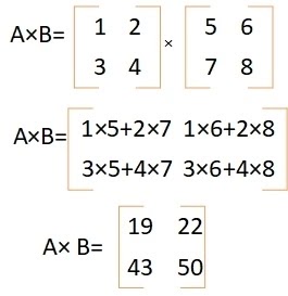
"While, to perform a matrix multiplications we can use the `@` operator as a shorthand for `np.matmul`.\n",
"\n",
"\n"
]
},
{
"cell_type": "code",
"execution_count": 23,
"id": "EtXbOvwrGJEB",
"metadata": {
"colab": {
"base_uri": "https://localhost:8080/"
},
"id": "EtXbOvwrGJEB",
"outputId": "4ffb241d-8d44-4b06-9f97-d1673bc969b1"
},
"outputs": [
{
"name": "stdout",
"output_type": "stream",
"text": [
"first matrix:\n",
"[[1 2]\n",
" [3 4]]\n",
"\n",
"second matrix:\n",
"[[5 6]\n",
" [7 8]]\n",
"\n",
"Matrix product:\n",
"[[19 22]\n",
" [43 50]]\n"
]
}
],
"source": [
"# Matrix multiplication using the @ operator\n",
"matrix_a = np.array([[1, 2], [3, 4]])\n",
"matrix_b = np.array([[5, 6], [7, 8]])\n",
"\n",
"print(f\"first matrix:\\n{matrix_a}\\n\\nsecond matrix:\\n{matrix_b}\\n\")\n",
"\n",
"matrix_product = matrix_a @ matrix_b\n",
"print(f\"Matrix product:\\n{matrix_product}\")"
]
},
{
"cell_type": "markdown",
"id": "pVbpA6KUDpam",
"metadata": {
"id": "pVbpA6KUDpam"
},
"source": [
"### Data Cleaning and Processing with NumPy\n",
"\n",
"Now we explore various techniques for data cleaning and processing using `NumPy`.\\\n",
"Let's start by creating a sample data with some missing values ( `np.nan `) and potential outliers."
]
},
{
"cell_type": "code",
"execution_count": 15,
"id": "S1YsPS9aFENk",
"metadata": {
"colab": {
"base_uri": "https://localhost:8080/"
},
"id": "S1YsPS9aFENk",
"outputId": "336e40d5-f976-405f-a26f-10312c55896f"
},
"outputs": [
{
"name": "stdout",
"output_type": "stream",
"text": [
"Original Data:\n",
"[ 1. 1.5 1.8 1.9 1.9 121.5 2. 2.1 2.2 2.2 2.3 2.5\n",
" 2.9 3.1 3.5 nan 4.2 100. 3.8 nan 2.7]\n"
]
}
],
"source": [
"# Create sample data\n",
"data = np.array([1.0, 1.5, 1.8, 1.9, 1.9, 121.5, 2.0, 2.1, 2.2, 2.2, 2.3, 2.5, 2.9, 3.1, 3.5, np.nan, 4.2, 100.0, 3.8, np.nan, 2.7])\n",
"\n",
"print(f\"Original Data:\\n{data}\")"
]
},
{
"cell_type": "markdown",
"id": "GGhSmb3-G8cw",
"metadata": {
"id": "GGhSmb3-G8cw"
},
"source": [
"Usually most of sensed data might have several missing values and outliers.\\\n",
"To identify those problematic elements in our dataset we can use some `Numpy` tools.\\\n",
"For missing data identification we can use `np.isnan`, crucial for understanding the extent and location of missing data before applying any cleaning techniques."
]
},
{
"cell_type": "code",
"execution_count": 16,
"id": "WUvAct1rHkIn",
"metadata": {
"colab": {
"base_uri": "https://localhost:8080/"
},
"id": "WUvAct1rHkIn",
"outputId": "17c71b11-4bdc-43be-d23e-c068edc1c6e9"
},
"outputs": [
{
"name": "stdout",
"output_type": "stream",
"text": [
"Missing Data Mask:[False False False False False False False False False False False False\n",
" False False False True False False False True False]\n",
"\n",
"Number of missing values:2\n"
]
}
],
"source": [
"# Identifying missing values (Binary NaN mask)\n",
"missing_mask = np.isnan(data)\n",
"print(f\"Missing Data Mask:{missing_mask}\\n\")\n",
"\n",
"# Counting missing values\n",
"num_missing = np.sum(missing_mask)\n",
"print(f\"Number of missing values:{num_missing}\")"
]
},
{
"cell_type": "markdown",
"id": "nA_ofPqPIUpF",
"metadata": {
"id": "nA_ofPqPIUpF"
},
"source": [
"After missing values identification, we can handle them by either replacing them with a specific value or using more fancy techniques.\\\n",
"We can try two different approaches:\n",
"- using `np.nan_to_num` to replace `np.nan` with 0,\n",
"- using `np.where` along with `np.nanmean` to replace missing values with the mean of the non-missing data.\n"
]
},
{
"cell_type": "code",
"execution_count": 17,
"id": "m_4Qj48hJAZz",
"metadata": {
"colab": {
"base_uri": "https://localhost:8080/"
},
"id": "m_4Qj48hJAZz",
"outputId": "d005b27b-3685-4617-981e-3b425f4dc812"
},
"outputs": [
{
"name": "stdout",
"output_type": "stream",
"text": [
"Data after replacing missing values with 0:\n",
"[ 1. 1.5 1.8 1.9 1.9 121.5 2. 2.1 2.2 2.2 2.3 2.5\n",
" 2.9 3.1 3.5 0. 4.2 100. 3.8 0. 2.7]\n",
"\n",
"The data mean value is:\n",
"13.85\n",
"Data after replacing missing values with the mean:\n",
"[ 1. 1.5 1.8 1.9 1.9 121.5 2. 2.1 2.2 2.2\n",
" 2.3 2.5 2.9 3.1 3.5 13.85 4.2 100. 3.8 13.85\n",
" 2.7 ]\n"
]
}
],
"source": [
"# Replacing np.nan with \"0\" using np.nan_to_num\n",
"data_filled = np.nan_to_num(data, nan=0.0)\n",
"print(f\"Data after replacing missing values with 0:\\n{data_filled}\\n\")\n",
"\n",
"# Replace np.nan with the rounded mean of non-missing values using np.nanman\n",
"mean_value = round(np.nanmean(data),2)\n",
"data_mean_filled = np.where(np.isnan(data), mean_value, data)\n",
"print(f\"The data mean value is:\\n{mean_value}\")\n",
"print(f\"Data after replacing missing values with the mean:\\n{data_mean_filled}\")"
]
},
{
"cell_type": "markdown",
"id": "7AGbzUN0MMEU",
"metadata": {
"id": "7AGbzUN0MMEU"
},
"source": [
"Data can often contain outliers that may skew the analysis.\\\n",
"In the previous example we can clearly see how the mean value was altered by outliers presence.\\\n",
"So we have to deal with data filtering or replacing in order to cut out such outliers.\\\n",
"One method consist in using a boolean indexing.\\\n",
"For example, we define a threshold and remove data points that exceed this value."
]
},
{
"cell_type": "code",
"execution_count": 18,
"id": "0z3yQb7aMzg2",
"metadata": {
"colab": {
"base_uri": "https://localhost:8080/"
},
"id": "0z3yQb7aMzg2",
"outputId": "ed3adb2b-5415-4607-9646-2854156a720a"
},
"outputs": [
{
"name": "stdout",
"output_type": "stream",
"text": [
"Data after filtering out outliers (values >= 20):\n",
"[1. 1.5 1.8 1.9 1.9 2. 2.1 2.2 2.2 2.3 2.5 2.9 3.1 3.5 4.2 3.8 2.7]\n"
]
}
],
"source": [
"# Definition of an outlier threshold (e.g., values >= 20 are considered outliers)\n",
"threshold = 20\n",
"filtered_data = data[data < threshold]\n",
"\n",
"print(f\"Data after filtering out outliers (values >= 20):\\n{filtered_data}\")"
]
},
{
"cell_type": "markdown",
"id": "QtOdwZmFOUBU",
"metadata": {
"id": "QtOdwZmFOUBU"
},
"source": [
"Another common data handling processing tasks consist in sorting and aggregation.\\\n",
"For this tasks we can use `np.sort` to order the data and `np.unique` to find distinct values; along with the calculation of the basic aggregate statistics like the sum (`np.sum`) and mean (`np.mean`) of the cleaned data.\n"
]
},
{
"cell_type": "code",
"execution_count": 20,
"id": "56bQtRhwQOv7",
"metadata": {
"colab": {
"base_uri": "https://localhost:8080/"
},
"id": "56bQtRhwQOv7",
"outputId": "92c4e2bf-05b0-4aa9-c3f2-4991101cf9f1"
},
"outputs": [
{
"name": "stdout",
"output_type": "stream",
"text": [
"Sorted Data:\n",
"[1. 1.5 1.8 1.9 1.9 2. 2.1 2.2 2.2 2.3 2.5 2.7 2.9 3.1 3.5 3.8 4.2]\n",
"Unique Values:\n",
"'[1. 1.5 1.8 1.9 2. 2.1 2.2 2.3 2.5 2.7 2.9 3.1 3.5 3.8 4.2]\n",
"\n",
"Sum: 41.6 \n",
"Mean: 2.45 \n",
"Std: 0.81\n"
]
}
],
"source": [
"# Sort the data after filling missing values\n",
"sorted_data = np.sort(filtered_data)\n",
"print(f\"Sorted Data:\\n{sorted_data}\")\n",
"\n",
"# Identify unique values\n",
"unique_values = np.unique(filtered_data)\n",
"print(f\"Unique Values:\\n'{unique_values}\")\n",
"\n",
"# Calculate aggregate statistics\n",
"data_sum = round(np.sum(filtered_data),2)\n",
"data_mean = round(np.mean(filtered_data),2)\n",
"data_std = round(np.std(filtered_data),2)\n",
"print('\\n\\\n",
"Sum:', data_sum, '\\n\\\n",
"Mean:', data_mean, '\\n\\\n",
"Std:', data_std)"
]
},
{
"cell_type": "markdown",
"id": "gfWCkuDUSFs2",
"metadata": {
"id": "gfWCkuDUSFs2"
},
"source": [
"After a deep data exploring, we can eventually use some more advanced data processing techniques.\\\n",
"One approach consist in using `np.where` for conditional data transformations with `np.clip` to limit the values within a specified range, which is often useful for handling extreme values."
]
},
{
"cell_type": "code",
"execution_count": 29,
"id": "bWAM_uazSrzq",
"metadata": {
"colab": {
"base_uri": "https://localhost:8080/"
},
"id": "bWAM_uazSrzq",
"outputId": "1f5249fa-269f-4c87-fc68-1a0b24cf4e5e"
},
"outputs": [
{
"name": "stdout",
"output_type": "stream",
"text": [
"Data after conditional processing (values < 3 multiplied by 10):\n",
"[ 1. 1.5 1.8 1.9 1.9 2. 2.1 2.2 2.2 2.3 2.5 2.9\n",
" 310. 350. 420. 380. 2.7]\n",
"Data after clipping values to the range 0-3:\n",
"'[1. 1.5 1.8 1.9 1.9 3. 2. 2.1 2.2 2.2 2.3 2.5 2.9 3. 3. 1. 3. 3.\n",
" 3. 1. 2.7]\n"
]
}
],
"source": [
"# Conditional processing example: data gain by multiply values > than 3 by 100\n",
"condition = filtered_data > 3\n",
"data_processed = np.where(condition, filtered_data * 100, filtered_data)\n",
"print(f\"Data after conditional processing (values < 3 multiplied by 100):\\n{data_processed}\")\n",
"\n",
"# Data ranging using np.clip to limit values to a range (e.g., 1 to 3)\n",
"data_clipped = np.clip(data_filled, 1, 3)\n",
"print(f\"Data after clipping values to the range 0-3:\\n'{data_clipped}\")"
]
},
{
"cell_type": "markdown",
"id": "O-dWn-BDUPNT",
"metadata": {
"id": "O-dWn-BDUPNT"
},
"source": [
"These `Numpy` tools, along with many others, are essential for manipulating and processing numerical data, expecially when those are (often) very large.\\\n",
"However, all techniques and methodologies that can potentially be employed in data processing must always be calibrated to the used data.\\\n",
"They need to fit the type of examinated data and the general purpose of these processings."
]
},
{
"cell_type": "markdown",
"id": "55758551-3cab-4ed7-b964-9dcc7898f041",
"metadata": {
"id": "55758551-3cab-4ed7-b964-9dcc7898f041"
},
"source": [
"## 5 - Pandas Basics\n",
"\n",
"\n",
"\n",
"Now we will explore `Pandas`, a powerful open-source library built on top of `NumPy`, widely used for data manipulation and analysis.\n",
"It introduces DataFrames and Series, which are highly efficient for working with tabular data.\n",
"\n",
"In this section, we cover:\n",
"- Basic functionality of the library,\n",
"- DataFrames and tools for exploration,\n",
"- Creating and manipulating Pandas Series and DataFrames,\n",
"- Data cleaning and standardization functionalities,\n",
"- Data importing and manipulatng from structured file formats,\n",
"- Basic data exploration and summary statistics\n"
]
},
{
"cell_type": "markdown",
"id": "Q8ow19NaSKyZ",
"metadata": {
"id": "Q8ow19NaSKyZ"
},
"source": [
"In Pandas we can create two main kind of data structure:\n",
"- **Pandas Series** (1D labeld array);\n",
"- **Pandas DataFrame** (2D labeled data structure).\n",
"\n",
"Both have the potential of having different types per cell/columns.\\\n",
"Pandas also offers a variety of tools for exploring data, such as `head()`, `tail()`, and `info()`, which help understand the dataset quickly.\n"
]
},
{
"cell_type": "code",
"execution_count": 23,
"id": "ey9by78hSRcA",
"metadata": {
"colab": {
"base_uri": "https://localhost:8080/"
},
"id": "ey9by78hSRcA",
"outputId": "1796c6ce-c665-4cf4-875b-d9341f66df17"
},
"outputs": [
{
"name": "stdout",
"output_type": "stream",
"text": [
"Pandas Series:\n",
"0 1\n",
"1 a\n",
"2 3\n",
"3 b\n",
"4 5\n",
"dtype: object\n"
]
}
],
"source": [
"# Creating a Pandas Series\n",
"series = pd.Series([1, \"a\", 3, \"b\", 5])\n",
"print(f\"Pandas Series:\\n\\\n",
"{series}\")\n"
]
},
{
"cell_type": "code",
"execution_count": 31,
"id": "bSdWA0tcd8L4",
"metadata": {
"colab": {
"base_uri": "https://localhost:8080/",
"height": 258
},
"id": "bSdWA0tcd8L4",
"outputId": "55c301f3-bea5-44ef-fe06-1211da4e23f5"
},
"outputs": [
{
"name": "stdout",
"output_type": "stream",
"text": [
"Same Pandas series seen with the enhanced Pandas data visualizzation:\n"
]
},
{
"data": {
"text/plain": [
"0 1\n",
"1 a\n",
"2 3\n",
"3 b\n",
"4 5\n",
"dtype: object"
]
},
"execution_count": 31,
"metadata": {},
"output_type": "execute_result"
}
],
"source": [
"print(\"Same Pandas series seen with the enhanced Pandas data visualizzation:\")\n",
"series"
]
},
{
"cell_type": "markdown",
"id": "nKF4LE9c_s17",
"metadata": {
"id": "nKF4LE9c_s17"
},
"source": [
"### Pandas Series\n",
"**Series** are easily explorable with the pandas tools to obtain information about the content of the data.\\\n",
"For instance, we can explore the Series with a simple loop, using `enumerate(series.items())` to extrapolate positions and values of some cells, also posing some particular conditions.\\\n",
"Or we can use `series.apply` to apply a `lambda x` function, as a small anonymous function inside another function for retrieving data.\\\n",
"In this case is inside `isinstance()` function, that returns `True` if the specified object is of the specified type, otherwise `False`.\\\n",
"In this way we can point out specific data or outliers by type or other conditions."
]
},
{
"cell_type": "code",
"execution_count": 24,
"id": "trjWKoBTaBii",
"metadata": {
"colab": {
"base_uri": "https://localhost:8080/"
},
"id": "trjWKoBTaBii",
"outputId": "952be8d9-4166-4ad4-86a9-1a7beb5051f9"
},
"outputs": [
{
"name": "stdout",
"output_type": "stream",
"text": [
"Series total length:\n",
"5\n",
"\n",
"Series type and position analysis:\n",
"Position: 0, Value: 1, Type: \n",
"Position: 1, Value: a, Type: \n",
"Position: 2, Value: 3, Type: \n",
"Position: 3, Value: b, Type: \n",
"Position: 4, Value: 5, Type: \n",
"\n",
"Number of strings cells:2\n",
"\n",
"Position of strings cells:\n",
"1 a\n",
"3 b\n",
"dtype: object\n",
"\n",
"Number of integers cells:3\n",
"\n",
"Position of integers cells:\n",
"0 1\n",
"2 3\n",
"4 5\n",
"dtype: object\n"
]
}
],
"source": [
"# Basic exploration and analysis of the Pd series\n",
"\n",
"print(f\"Series total length:\\n{len(series)}\\n\")\n",
"print(\"Series type and position analysis:\")\n",
"for i, (index, value) in enumerate(series.items()):\n",
" print(f\"Position: {index}, Value: {value}, Type: {type(value)}\")\n",
"\n",
"# Localization of specific cells\n",
"# Strings localization\n",
"strings = series.apply(lambda x: isinstance(x, str))\n",
"print(f\"\\nNumber of strings cells:{len(series[strings])}\")\n",
"print(\"\\nPosition of strings cells:\")\n",
"print(series[strings])\n",
"\n",
"\n",
"# Int localization\n",
"integers = series.apply(lambda x: isinstance(x, int))\n",
"print(f\"\\nNumber of integers cells:{len(series[integers])}\")\n",
"print(\"\\nPosition of integers cells:\")\n",
"print(series[integers])\n",
"\n"
]
},
{
"cell_type": "markdown",
"id": "l1_vpuZSGqCm",
"metadata": {
"id": "l1_vpuZSGqCm"
},
"source": [
"### Pandas DataFrame\n",
"Unlike the **Series**, a **DataFrame** is a 2D labeled data structure, widely used because it can have columns of different types.\\\n",
"It can be created:\n",
"- starting from a dictionary,\n",
"- populated row by row,\n",
"- by the combination of other dataframes or data structures.\n",
"\n",
"It offers a variety of tools for exploring data, such as `.head()`, `.tail()`,`.sort_index`, `.sort_value` and `.info()`, which help understand the dataset quickly.\""
]
},
{
"cell_type": "code",
"execution_count": 33,
"id": "uM-XkFQnZgd5",
"metadata": {
"colab": {
"base_uri": "https://localhost:8080/"
},
"id": "uM-XkFQnZgd5",
"outputId": "dddbcbcf-63ac-421a-8720-74145311ccc1"
},
"outputs": [
{
"name": "stdout",
"output_type": "stream",
"text": [
"Pandas dataframe:\n",
" Station AverageTemp (T°C) AverageUmidity (%)\n",
"0 S01 25.5 58\n",
"1 S02 26.1 67\n",
"2 S03 27.3 70\n",
"3 S04 25.8 61\n",
"4 S05 25.1 59\n",
"5 S06 24.9 55\n"
]
}
],
"source": [
"# Creating a DataFrame and Basic Exploration\n",
"# Create a DataFrame from a dictionary\n",
"data = {\n",
" 'Station': ['S01', 'S02', 'S03', 'S04','S05','S06'], #col1\n",
" 'AverageTemp (T°C)': [25.5, 26.1, 27.3, 25.8, 25.1, 24.9,], #col2\n",
" 'AverageUmidity (%)': [58, 67, 70, 61, 59, 55] #col3\n",
" }\n",
"\n",
"df = pd.DataFrame(data)\n",
"\n",
"print(f\"Pandas dataframe:\\n {df}\")"
]
},
{
"cell_type": "code",
"execution_count": 34,
"id": "SsawoUKQeI6k",
"metadata": {
"colab": {
"base_uri": "https://localhost:8080/",
"height": 255
},
"id": "SsawoUKQeI6k",
"outputId": "0537207f-96ad-4e1d-eb0f-ea2a2954c699"
},
"outputs": [
{
"name": "stdout",
"output_type": "stream",
"text": [
"Same Pandas dataframe seen with the enhanced Pandas data visualizzation:\n"
]
},
{
"data": {
"text/html": [
"\n",
"\n",
"
\n",
" \n",
" \n",
" | \n",
" Station | \n",
" AverageTemp (T°C) | \n",
" AverageUmidity (%) | \n",
"
\n",
" \n",
" \n",
" \n",
" | 0 | \n",
" S01 | \n",
" 25.5 | \n",
" 58 | \n",
"
\n",
" \n",
" | 1 | \n",
" S02 | \n",
" 26.1 | \n",
" 67 | \n",
"
\n",
" \n",
" | 2 | \n",
" S03 | \n",
" 27.3 | \n",
" 70 | \n",
"
\n",
" \n",
" | 3 | \n",
" S04 | \n",
" 25.8 | \n",
" 61 | \n",
"
\n",
" \n",
" | 4 | \n",
" S05 | \n",
" 25.1 | \n",
" 59 | \n",
"
\n",
" \n",
" | 5 | \n",
" S06 | \n",
" 24.9 | \n",
" 55 | \n",
"
\n",
" \n",
"
\n",
"
\n",
"\n",
"
\n",
" \n",
" \n",
" | \n",
" DATA | \n",
" TM | \n",
" UM | \n",
" VVM | \n",
" PRE | \n",
" RSM | \n",
" PATM | \n",
" QA PS PM | \n",
" QA PG PM | \n",
" ORA | \n",
"
\n",
" \n",
" \n",
" \n",
" | 0 | \n",
" 03/12/2021 | \n",
" 7,420 | \n",
" 95,300 | \n",
" 2,750 | \n",
" 0,250 | \n",
" 24,6 | \n",
" 951 | \n",
" 0,500 | \n",
" 0,150 | \n",
" 12:00 | \n",
"
\n",
" \n",
" | 1 | \n",
" 04/12/2021 | \n",
" 9,490 | \n",
" 72,600 | \n",
" 3,590 | \n",
" 0,000 | \n",
" 35,9 | \n",
" 957 | \n",
" 0,530 | \n",
" 0,000 | \n",
" 12:00 | \n",
"
\n",
" \n",
" | 2 | \n",
" 05/12/2021 | \n",
" 11,900 | \n",
" 79,900 | \n",
" 3,970 | \n",
" 0,000 | \n",
" 38,4 | \n",
" 952 | \n",
" 0,040 | \n",
" 0,010 | \n",
" 12:00 | \n",
"
\n",
" \n",
" | 3 | \n",
" 06/12/2021 | \n",
" 7,400 | \n",
" 85,800 | \n",
" 2,120 | \n",
" 0,000 | \n",
" 185,0 | \n",
" 947 | \n",
" 0,000 | \n",
" 0,000 | \n",
" 12:00 | \n",
"
\n",
" \n",
" | 4 | \n",
" 07/12/2021 | \n",
" 6,480 | \n",
" 72,900 | \n",
" 4,980 | \n",
" 0,000 | \n",
" 320,0 | \n",
" 952 | \n",
" 0,140 | \n",
" 0,100 | \n",
" 12:00 | \n",
"
\n",
" \n",
" | ... | \n",
" ... | \n",
" ... | \n",
" ... | \n",
" ... | \n",
" ... | \n",
" ... | \n",
" ... | \n",
" ... | \n",
" ... | \n",
" ... | \n",
"
\n",
" \n",
" | 200 | \n",
" 05/08/2022 | \n",
" 33,500 | \n",
" 21,200 | \n",
" 1,670 | \n",
" 0,000 | \n",
" 794,0 | \n",
" 960 | \n",
" 1,020 | \n",
" 0,900 | \n",
" 12:00 | \n",
"
\n",
" \n",
" | 201 | \n",
" 06/08/2022 | \n",
" ND | \n",
" ND | \n",
" ND | \n",
" ND | \n",
" ND | \n",
" ND | \n",
" ND | \n",
" ND | \n",
" 12:00 | \n",
"
\n",
" \n",
" | 202 | \n",
" 07/08/2022 | \n",
" ND | \n",
" ND | \n",
" ND | \n",
" ND | \n",
" ND | \n",
" ND | \n",
" ND | \n",
" ND | \n",
" 12:00 | \n",
"
\n",
" \n",
" | 203 | \n",
" 08/08/2022 | \n",
" ND | \n",
" ND | \n",
" ND | \n",
" ND | \n",
" ND | \n",
" ND | \n",
" ND | \n",
" ND | \n",
" 12:00 | \n",
"
\n",
" \n",
" | 204 | \n",
" 10/08/2022 | \n",
" 27,100 | \n",
" 53,500 | \n",
" 4,400 | \n",
" 0,000 | \n",
" 533,0 | \n",
" 961,0 | \n",
" 1,370 | \n",
" 1,500 | \n",
" 12:00 | \n",
"
\n",
" \n",
"
\n",
"
205 rows × 10 columns
\n",
"
\n",
"\n",
"
\n",
" \n",
" \n",
" | Season | \n",
" Autunno | \n",
" Estate | \n",
" Inverno | \n",
" Primavera | \n",
"
\n",
" \n",
" | Region | \n",
" | \n",
" | \n",
" | \n",
" | \n",
"
\n",
" \n",
" \n",
" \n",
" | Basilicata | \n",
" 16 | \n",
" 25 | \n",
" 5 | \n",
" 12 | \n",
"
\n",
" \n",
" | Molise | \n",
" 14 | \n",
" 24 | \n",
" 3 | \n",
" 10 | \n",
"
\n",
" \n",
" | Puglia | \n",
" 18 | \n",
" 27 | \n",
" 8 | \n",
" 15 | \n",
"
\n",
" \n",
"
\n",
"